Understanding Polynomial Functions: A Comprehensive Guide For Analysis And Manipulation

To write a polynomial function, begin with monomials (terms with a variable raised to a power). Polynomials combine multiple monomials, classified as binomials (two terms) or trinomials (three terms). The degree reflects the highest exponent, with the leading coefficient accompanying the highest-degree term. As functions, polynomials can be transformed or graphed. Their end behavior (long-term trends) depends on the degree and leading coefficient. Factor and remainder theorems facilitate root (zero) identification and evaluating polynomials, providing insights into polynomial functions’ structure and behavior.

Monomials: The Basic Bricks of Polynomials

• Define monomials and their components (term, coefficient, variable)
• Provide examples to illustrate the concept

Monomials: The Fundamental Building Blocks of Polynomials

Polynomials, the mathematical expressions that form the foundation of algebra, are composed of a fundamental unit known as the monomial. Understanding monomials is the cornerstone for comprehending the intricacies of polynomials.

A monomial is an expression that consists of a term, a coefficient, and a variable. The term is a mathematical operation (e.g., multiplication or division) involving the variable, while the coefficient is the number multiplied by the variable. The variable is the unknown quantity in the expression.

For example, consider the monomial 3x². Here, 3 is the coefficient, x is the variable, and x² is the term. The coefficient tells us that the variable is multiplied by itself three times.

Monomials are the basic building blocks of polynomials. Just as bricks can be used to construct intricate structures, monomials can be combined to form more complex polynomials. By comprehending the concept of monomials, we lay the groundwork for understanding the fascinating world of polynomials and their applications in mathematics and beyond.

Polynomials: Expressions with Multiple Terms

Polynomials are like advanced versions of monomials, which are simply single terms made up of a coefficient (a number), a variable (a letter representing an unknown value), and an exponent (the power to which the variable is raised). When we combine multiple monomials, we get a polynomial.

Polynomials consist of terms, which are individual monomials. Each term in a polynomial has its own coefficient and variable. Just like monomials, polynomials also have a degree, which is the highest exponent of any variable in the polynomial.

Polynomials can be classified into different types based on the number of terms. Binomials have two terms, while trinomials have three terms. For example, “2x + 5” is a binomial, and “x² – 3x + 2” is a trinomial.

Understanding polynomials is crucial in algebra and beyond. They are used in functions, calculus, and many other areas of mathematics and science. By delving deeper into the world of polynomials, you’ll unlock powerful tools for exploring the complexities of the universe.

Degree and Leading Coefficient: Markers of Polynomial Structure

• Explain degree as the highest exponent of the variable
• Define the leading coefficient as the coefficient with the highest exponent

Degree and Leading Coefficient: Navigating the Maze of Polynomials

In the realm of mathematics, polynomials stand tall as expressions composed of multiple terms. Each term in this intricate mosaic is known as a monomial, the building block of these mathematical structures. Understanding the degree and leading coefficient of a polynomial is like deciphering the blueprint that shapes its behavior.

Degree: The Highest Power at Play

Think of the degree of a polynomial as the highest exponent of the variable within the expression. This numerical value signifies the polynomial’s complexity and determines its overall curvature. For instance, if the variable (x) is raised to the power of 5, the polynomial has a degree of 5.

Leading Coefficient: Guiding the Polynomial’s Path

Amidst the polynomial’s tapestry, the leading coefficient emerges as the coefficient of the term with the highest exponent. It plays a pivotal role in determining the polynomial’s characteristics, such as its slope, concavity, and overall shape. A positive leading coefficient indicates that the polynomial rises as the variable increases, while a negative leading coefficient suggests a downward trajectory.

Interplay of Degree and Leading Coefficient: Unlocking Polynomial Behavior

Together, the degree and leading coefficient provide a comprehensive roadmap for comprehending a polynomial’s behavior. A high degree implies greater complexity and potential oscillations, while a large leading coefficient amplifies the polynomial’s curvature. Conversely, a low degree signifies a simpler structure, and a small leading coefficient results in a more gentle curve.

Polynomials as Functions: Exploring Transformations and Graphing

Unveiling the Power of Functions

In the realm of mathematics, functions play a pivotal role in describing relationships between variables. These relationships can be visualized through graphs, providing valuable insights into the behavior of the function. Polynomials, as expressions consisting of multiple terms, exhibit fascinating functional properties that allow us to manipulate and graph them effortlessly.

Introducing Parent Functions

Every polynomial function has a corresponding parent function that serves as a template for its behavior. The parent function of a linear polynomial, for example, is y = x. It represents a straight line passing through the origin with a slope of 1. Similarly, the parent function of a quadratic polynomial is y = x², which forms a parabola opening upwards with a vertex at the origin.

Transforming Functions: A Visual Symphony

Polynomials can be transformed by applying a range of operations that modify their shape and position. Shifting involves moving the function up, down, left, or right. Dilation changes the function’s size, either vertically or horizontally. Reflection flips the function across the x- or y-axis.

These transformations can drastically alter the appearance of a polynomial function. By combining different transformations, we can create an infinite variety of graphs representing complex relationships between variables.

Translating Knowledge into Graphs

Understanding the transformations applied to a polynomial function empowers us to predict its graph. For instance, the graph of y = x² – 3 can be obtained by shifting the parent function y = x² down by 3 units. This transformation produces a parabola with the same shape but located lower on the coordinate plane.

Polynomials, as functions, offer a powerful tool for representing and analyzing relationships between variables. By mastering the art of transformations, we can manipulate polynomial functions to create graphs that accurately depict the underlying mathematical patterns. This understanding forms the foundation for solving complex problems and unraveling the secrets of the mathematical world.

End Behavior: Analyzing Long-Term Trends

• Define end behavior and its relation to asymptotes and limits
• Show how to determine end behavior based on degree and leading coefficient

End Behavior: Unraveling the Long-Term Story of Polynomials

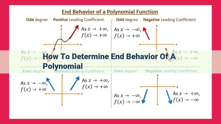
In the realm of polynomials, a profound concept known as end behavior unveils the long-term trends of these algebraic expressions. It reveals how they behave as the variable approaches infinity or negative infinity. This understanding is crucial for graphing and analyzing polynomials.

End behavior is closely intertwined with two mathematical concepts: asymptotes and limits. Asymptotes are lines that a polynomial approaches but never touches, while limits describe the value a function approaches as the variable changes without bound. By understanding the relationship between these ideas, we can determine the end behavior of polynomials.

The degree of a polynomial determines its end behavior. A polynomial with an even degree will have end behavior that oscillates around an asymptote, while a polynomial with an odd degree will have end behavior that approaches infinity or negative infinity. The leading coefficient, which is the coefficient of the term with the highest exponent, also plays a role. If the leading coefficient is positive, the polynomial will increase or decrease without bound, depending on its degree. If it’s negative, the function will decrease or increase without bound.

Here’s a simple example to illustrate:

Consider the polynomial f(x) = x^2 + 2x – 3. Its degree is 2, which is even, and its leading coefficient is 1, which is positive. Therefore, as x approaches infinity, f(x) approaches positive infinity. Conversely, as x approaches negative infinity, f(x) also approaches positive infinity. This is because the x^2 term dominates the polynomial as x becomes very large, and the x^2 term increases without bound.

**Unveiling the Roots of Polynomials: The Factor Theorem Demystified**

In the realm of polynomials, there lies a powerful tool known as the Factor Theorem, an invaluable aid in unearthing the enigmatic roots that govern their behavior. Let us embark on a journey to unravel this theorem and embrace its potency in deciphering polynomial secrets.

The Factor Theorem: A Path to Divisibility

The Factor Theorem unveils a profound connection between polynomials and their roots. It asserts that a polynomial, f(x), is divisible by (x – a) if and only if “a” is a root of f(x). This remarkable testament opens the door to uncovering the hidden roots that shape a polynomial’s destiny.

Harnessing the Factor Theorem: Finding Roots with Precision

To harness the power of the Factor Theorem, we embark on a methodical process:

1. Substitute the alleged root (a) into f(x).
2. Evaluate f(a).
3. If f(a) = 0, then “a” is indeed a root of the polynomial.

This simple yet potent procedure empowers us to pinpoint the roots of polynomials with remarkable accuracy.

A Deeper Dive: The Broader Significance of the Factor Theorem

The Factor Theorem extends far beyond its utility as a mere root-finding tool. It finds applications in:

• Simplifying Expressions: By factoring polynomials using the Factor Theorem, we can simplify complex expressions and unveil their underlying patterns.
• Solving Equations: Roots provide essential clues in solving polynomial equations, and the Factor Theorem serves as a catalyst in this endeavor.
• Graphing Polynomials: The location of roots determines the shape and behavior of polynomial graphs, making the Factor Theorem a vital tool in predicting their characteristics.

In conclusion, the Factor Theorem stands as a formidable ally in our mathematical pursuits. It empowers us to unravel the mysteries that lie within polynomials, revealing their intricate structure and enabling us to manipulate them with newfound precision. Embrace the Factor Theorem, and unlock the secrets that lie dormant in the realm of polynomials.

The Remainder Theorem: Unveiling the Secrets of Division

In the realm of polynomials, the remainder theorem emerges as a powerful tool that sheds light on the intricate relationship between division and remainders. This theorem provides a fundamental understanding of how to navigate polynomial division and evaluate polynomials with ease.

Imagine we have a polynomial p(x) and a divisor d(x) ≠ 0. When we divide p(x) by d(x), we obtain a quotient q(x) and a remainder r(x). The remainder theorem states that the remainder r(x) when p(x) is divided by d(x) is equal to p(c), where c is the constant term of d(x).

This profound revelation enables us to derive a myriad of valuable insights into polynomials. For instance, it simplifies the task of finding remainders. To determine the remainder when p(x) is divided by d(x), simply substitute the constant term of d(x) into p(x) and evaluate the result. This straightforward approach eliminates the need for long division.

Furthermore, the remainder theorem empowers us to evaluate polynomials swiftly and accurately. By substituting a specific value for x into p(x), we can readily determine the value of p(x). This technique proves particularly useful when dealing with polynomials of higher degrees, where direct evaluation becomes cumbersome.

In essence, the remainder theorem provides a bridge between division and evaluation, offering a profound understanding of polynomial operations. Its applications extend far beyond theoretical insights, enabling us to tackle real-world problems with confidence and efficiency.