Understanding Polynomial Function Roots: Number, Multiplicities, And Impact On Graph

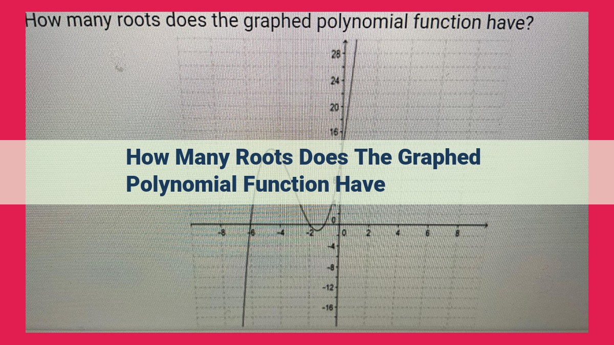
A graphed polynomial function can have multiple roots, which are the values of the variable at which the function crosses the x-axis. The number of roots is determined by the polynomial’s degree, which is the highest power of the variable in the function. In general, a polynomial of degree n has n roots. However, some roots may be complex (non-real) and not visible on the real number line. Additionally, roots can have varying multiplicities, which are indicated by their order of appearance in the factored form of the polynomial. Roots with higher multiplicities can affect the polynomial’s shape and behavior near those roots.

Explain the concept of factors, both real and complex

Understanding the Essence of Factors: Unveiling the Roots of Polynomials

Embarking on a mathematical adventure, we delve into the captivating realm of polynomials, where factors play a pivotal role in shaping these enigmatic expressions. Factors, like building blocks, are the fundamental components that determine the behavior and characteristics of polynomials. They can be real or complex, each with its unique properties and contributions.

Real factors are numbers that, when multiplied together, produce the polynomial. They can be positive or negative, and their relationship to the polynomial’s roots is particularly intriguing. Real roots are values of the variable that make the polynomial equal to zero when substituted. These roots emerge as the zeros of the polynomial, where it touches the x-axis.

Venturing beyond the realm of real numbers, we encounter imaginary roots, which reside in the imaginary plane. They are numbers that, when squared, produce a negative value. Imaginary roots typically appear in conjugate pairs, which possess the same absolute value but opposite signs. These complex roots play a crucial role in the analysis and understanding of polynomials.

By unraveling the intricate tapestry of factors and roots, we gain a deeper appreciation for the inner workings of polynomials. These concepts lay the foundation for exploring the fascinating connections between the coefficients, degree, and behavior of these mathematical expressions, unlocking a wealth of insights into their properties and applications.

Understanding Real Roots and Their Relationship to Real Factors

In the vast landscape of mathematics, polynomials hold a fascinating place, like enigmatic puzzles waiting to be solved. At their very core lie factors, the building blocks that shape their complexity. Real factors are like the tangible components, the solid foundation upon which the polynomial rests.

When a polynomial possesses real factors, it unveils a special connection to its roots. Roots, like invisible anchors, hold the polynomial in place, dictating its behavior and revealing its secrets. Real roots emerge when the polynomial’s value sinks to zero, like the moment of perfect balance on a seesaw.

The relationship between real factors and real roots is an intricate dance, a harmonious interplay that reveals the polynomial’s true nature. Real roots are like shadows cast by real factors, mirroring their presence in the polynomial’s equation. Each real factor whispers a hint, a clue to the polynomial’s underlying structure. By understanding this connection, we can unravel the polynomial’s mysteries and gain a deeper appreciation for its mathematical beauty.

Understanding Factors and Roots

Every polynomial equation has factors, which are like building blocks that make up the equation. These factors can be either real numbers or complex numbers, which involve the imaginary unit i.

Real Roots

Real roots are the numbers that make a polynomial equal to zero when plugged in. They are like the points where the polynomial crosses the x-axis. Real roots correspond to real factors. For example, the polynomial x^2 – 4 has two real roots, 2 and -2, which correspond to the factors (x – 2) and (x + 2).

Imaginary Roots

Imaginary roots are roots that involve the imaginary unit i. They are like points that lie on a vertical axis perpendicular to the real axis. Imaginary roots always come in conjugate pairs, meaning they are mirror images of each other across the real axis. For example, the polynomial x^2 + 1 has two imaginary roots, i and -i, which correspond to the conjugate pair of factors (x + i) and (x – i).

Degree and Roots: Unlocking the Number of Real Roots

Picture a polynomial, a mathematical expression consisting of variables and constants, like a roller coaster with multiple hills and valleys. The degree of a polynomial, akin to the height of the roller coaster, determines the number of potential real roots it possesses.

Just as a roller coaster with an even degree has an equal number of hills and valleys, a polynomial with an even degree will have an equal number of positive and negative real roots. Think of it as a balanced roller coaster ride, with every uphill matched by a downhill.

On the other hand, a polynomial with an odd degree behaves like a roller coaster with an odd number of hills and valleys. Such polynomials will always have at least one real root, like a roller coaster starting and ending at ground level. This is because the polynomial’s graph must cross the x-axis at least once.

Understanding the degree of a polynomial is the first step to unraveling its real roots, providing valuable insights into the polynomial’s behavior and shape.

Unlocking the Mysteries of Polynomials: Degrees and Roots

When exploring the fascinating world of polynomials, understanding their degrees and roots is crucial. Join us on a journey to unravel these secrets, starting with the role of polynomial degrees in determining the number of real roots.

A polynomial’s degree represents its highest exponent. Even-degree polynomials have an equal number of positive and negative roots, while odd-degree polynomials guarantee at least one real root. For instance, a quadratic polynomial (degree 2) can have two real roots, one positive and one negative.

Intriguingly, polynomials with odd degrees also promise at least one positive root. This is because the polynomial’s behavior at infinity is determined by its leading coefficient. A positive leading coefficient implies that the polynomial rises towards infinity, crossing the x-axis at least once and yielding a positive real root.

Unveiling the Leading Coefficient’s Power: Exploring Its Influence on the Polynomial’s Journey

Every journey begins with a first step, and for polynomials, that first step often lies in the leading coefficient. This mysterious force shapes the polynomial’s fate, guiding its path and determining its behavior at the very edge of infinity.

Imagine a polynomial as a vibrant line dancing across the coordinate plane. The leading coefficient is the choreographer who sets the line’s slope, dictating the angle at which it ascends or descends. At the point where the line intersects the y-axis, it’s like a snapshot of the polynomial’s journey and reveals the value of the y-intercept. This crucial point holds the key to understanding the polynomial’s initial position and its overall character.

Positive Coefficients: Soaring High

When the leading coefficient is positive, the polynomial starts its ascent like a rocket. The line slopes upward, eager to explore the realms of positive infinity. The y-intercept becomes a point of departure, marking the height from which the polynomial takes flight.

Negative Coefficients: Delving into Depths

In contrast, a negative leading coefficient sends the polynomial on a downward trajectory. The line plunges into the negative depths, diving towards minus infinity. The y-intercept becomes a point of despair, indicating the low point from which the polynomial begins its descent.

Magnitude Matters: Shaping the Curve

The magnitude of the leading coefficient also plays a vital role. A large positive or negative coefficient exaggerates the slope, creating a steeper curve. The line becomes more pronounced, and the polynomial’s journey becomes more dramatic.

So, next time you encounter a polynomial, remember the power wielded by its leading coefficient. It holds the blueprint for the polynomial’s journey, shaping its ascent or descent and determining its fate at infinity.

The Leading Coefficient’s Tale: Shaping the Polynomial’s Infinite Adventure

In the realm of polynomials, the leading coefficient stands as a majestic navigator, guiding the polynomial’s destiny as it embarks on its journey towards infinity.

Imagine a lone polynomial, its treacherous path stretching infinitely before it. As it ventures forth, the leading coefficient acts as its unwavering beacon, dictating its ultimate destination. A positive leading coefficient propels the polynomial upwards, its branches reaching ever higher towards the celestial expanse. Like an unrestrained comet, it soars indefinitely, never succumbing to the gravitational pull of the origin.

In contrast, a negative leading coefficient transforms the polynomial into a celestial diver, plunging it downwards with relentless force. Its branches dip below the horizon, swallowed by the abyss. As the polynomial ventures further into the depths, its shape becomes increasingly compressed, eventually vanishing into nothingness.

This interplay between the leading coefficient and the polynomial’s behavior at infinity unveils a profound truth: the leading coefficient holds the key to unlocking the polynomial’s asymptotic destiny. It determines whether the polynomial will soar to celestial heights or descend into an eternal abyss, shaping its fate for all eternity.

Describe how linear factors can contribute to roots

Unveiling the Roots: The Role of Linear Factors

Introduction:
In the realm of polynomials, roots hold a pivotal position. They represent the points where a polynomial’s graph intercepts the x-axis, offering valuable insights into the polynomial’s behavior. Linear factors play a crucial role in determining these roots.

Linear Factors and Roots:
Linear factors are first-degree polynomials that have the general form (x – a). When a linear factor is present in a polynomial, it contributes to the roots of that polynomial. Specifically, the value of ‘a’ in the linear factor corresponds to a root of the polynomial.

Contribution to Roots:
Let’s consider the polynomial f(x) = (x – 2)(x + 3). The linear factor (x – 2) contributes the root x = 2 to f(x). This means that the graph of f(x) intercepts the x-axis at x = 2. Similarly, the linear factor (x + 3) contributes the root x = -3.

Multiple Roots and Linear Factors:
In certain cases, multiple linear factors with the same value of ‘a’ can occur in a polynomial. These multiple linear factors correspond to multiple roots of the polynomial. For instance, in the polynomial f(x) = (x – 2)²(x + 1), the linear factor (x – 2) appears twice, indicating that x = 2 is a double root.

Understanding the Impact:
The presence of linear factors can significantly impact the shape and behavior of a polynomial’s graph. Roots associated with linear factors correspond to points where the graph crosses the x-axis. These points determine the intercepts and extrema of the graph, influencing its overall curvature and behavior.

Unveiling Roots from Linear Factors: A Journey into Polynomial Equations

In the realm of algebra, polynomials reign supreme, orchestrating intricate equations that can be untangled by understanding their hidden roots and factors. When a polynomial equation contains linear factors, it holds the key to uncovering specific roots that shape its behavior and reveal its secrets.

Identifying Linear Factors and Their Roots

Linear factors are the simplest building blocks of polynomials, consisting of a coefficient and a variable raised to the first power. To identify roots that correspond to linear factors, we embark on a detective journey, seeking clues within the equation.

Real Roots Unmasked

If a linear factor has a real coefficient and a positive constant, the root it corresponds to will also be real. For instance, in the polynomial equation 2x – 4, the linear factor is (2x – 4), and its root is 2, which is a real number.

Unveiling Imaginary Roots

However, when a linear factor has a real coefficient and a negative constant, things get a bit more intriguing. The root it corresponds to will be imaginary, denoted by the symbol i (√-1). For example, in the polynomial equation x² – 2x + 2, the linear factors are (x – 1 + i) and (x – 1 – i), and their roots are 1 + i and 1 – i, respectively, which are both imaginary numbers.

Conjugate Pairs: A Harmonic Dance

Imaginary roots always come in pairs known as conjugate pairs. These pairs have the same real part but differ in their imaginary part by a sign flip. For instance, in the previous example, the conjugate pair of roots is 1 + i and 1 – i.

By understanding how to identify roots that correspond to linear factors, we gain a deeper insight into the structure of polynomials and their intricate dance with real and imaginary numbers.

Diving Deeper into Root Multiplicity: Unraveling Polynomial Secrets

In our exploration of polynomials, we’ve stumbled upon the enigmatic concept of root multiplicity, a property that unveils the polynomial’s hidden behavior and shape. Imagine a captivating storyline where polynomials dance across the mathematical canvas, each with its unique characteristics, and root multiplicity serves as the choreographer, orchestrating their graceful movements.

Unraveling the Multiplicity Mystery

Root multiplicity refers to the number of times a particular root appears as a solution to the polynomial equation. It’s akin to a musical chord, where the same note can be played multiple times, each repetition enhancing its resonance. In polynomials, multiple roots paint a distinctive picture on the graph.

The Impact on the Graph

When a root has multiplicity n, the polynomial graph exhibits a captivating behavior at that root. The graph either:

• Crosses the x-axis tangentially: If n is even, the polynomial gently kisses the x-axis at the root, mirroring its smooth passage.
• Touches the x-axis with a sharp turn: If n is odd, the polynomial grazes the x-axis with a graceful arc, indicating a momentary pause at the root.

Revealing the Polynomial’s Shape

Root multiplicity also shapes the polynomial’s overall form. Higher multiplicity roots create flatter sections on the graph, while lower multiplicity roots result in sharper peaks or valleys. This subtle interplay of multiplicity and graph shape paints a unique silhouette for each polynomial.

Unveiling the Polynomial’s Nature

By unraveling root multiplicity, we gain insight into the polynomial’s character. High-order multiplicity roots betray a polynomial that stubbornly clings to the x-axis, while low-order multiplicity roots suggest a polynomial that prefers a more dynamic dance across the coordinate plane.

In essence, root multiplicity is the secret code that orchestrates the intricate behavior and shape of polynomials. By deciphering this code, we unlock a deeper understanding of these mathematical masterpieces.

Multiplicity of Roots: Unveiling the Polynomial’s Behavior and Shape

Imagine you have a beautiful vase, but its handle has a pesky crack. If you slightly touch the crack, it might only cause a small vibration. However, if you press down hard on the same crack, the vase might shatter into a million pieces. Similarly, the behavior and shape of a polynomial are influenced by the multiplicity of its roots.

• Roots and Graphing: Each root of a polynomial represents a point where the graph crosses the x-axis. A root of multiplicity 1 corresponds to a single crossing point, creating a simple “bump” or “dip” in the graph.
• Double the Multiplicity, Double the Impact: When a polynomial has a root of multiplicity 2, the graph “bounces” off the x-axis at that point. It touches the axis but doesn’t cross over, creating a “V” or “U” shape.
• Triple the Fun, Triple the Tangency: A root of multiplicity 3 results in the graph “kissing” the x-axis, rather than crossing or bouncing. It touches the axis and has a flat slope, forming a “W” or “M” shape.

The higher the root’s multiplicity, the flatter the graph becomes at the crossing point. This means that the polynomial’s behavior is less reactive to changes in the input value. For example, a polynomial with a root of multiplicity 5 will exhibit a very gradual change in slope near the crossing point.

Summary:

The multiplicity of roots in a polynomial profoundly impacts its graph’s shape and behavior. Roots of higher multiplicity create more pronounced “bumps,” “dips,” or flattened regions where the graph interacts with the x-axis. Understanding root multiplicity is essential for analyzing and understanding the characteristics of any given polynomial.