Understanding Orthogonality And Its Applications In Linear Algebra

Orthogonal vectors are perpendicular to each other, meaning their dot product is zero. The Gram-Schmidt process is a method for generating orthogonal vectors from a set of linearly independent vectors. It involves subtracting projections of each vector onto previously found orthogonal vectors. A conjugate orthogonal basis is a set of mutually orthogonal vectors that span the same vector space as the original set. The orthogonal complement subspace is the set of all vectors orthogonal to a given subspace. To find an orthogonal vector to a given vector, you can use the Gram-Schmidt process or calculate the projection of the given vector onto the orthogonal complement subspace.

Unveiling the Secrets of Orthogonal Vectors: A Path to Linear Algebra Mastery

In the realm of vector spaces, the concept of orthogonality reigns supreme, offering a crucial foundation for many mathematical endeavors. Orthogonal vectors, like harmonious notes in a melody, are perpendicular to each other, creating a symphony of linear independence.

To delve into this concept, let’s begin with its definition. Orthogonality arises when two vectors, say u and v, satisfy a crucial condition: their dot product is zero. The dot product, denoted as u · v, measures the extent to which vectors u and v align with or oppose each other. If their dot product vanishes, it signifies that they are perpendicular, or in other words, orth ogonal.

The significance of orthogonality extends far beyond its geometric interpretation. In vector spaces, orthogonal vectors form the cornerstone of many applications, including:

• Linear independence: Orthogonal vectors cannot be linearly combined to create any other vector in the space, ensuring their uniqueness and freedom from redundancy.
• Basis vectors: A set of orthogonal vectors can serve as a basis for the vector space, providing a convenient and efficient way to describe any vector within it.
• Coordinate systems: Orthogonal vectors form the axes of coordinate systems, allowing us to locate and manipulate vectors in a structured manner.

Understanding orthogonal vectors is thus essential for navigating the complexities of vector spaces and unlocking their full potential in applications such as physics, engineering, and computer graphics.

The Gram-Schmidt Process: A Step-by-Step Guide to Creating Orthogonal Vectors

Imagine you have a collection of vectors that point in all different directions. How can you transform them into a set of vectors that are all perpendicular to each other? This is where the Gram-Schmidt process comes in. It’s a mathematical tool that allows you to create a set of orthogonal vectors, which are vectors that form right angles with each other.

Step-by-Step Process

The Gram-Schmidt process involves a series of steps:

1. Normalize the first vector. Normalize means to scale the vector to have a length of 1. This creates a unit vector.
2. Project all other vectors onto the first unit vector. This gives you a set of orthogonal projections.
3. Subtract the orthogonal projections from the original vectors. This results in a set of vectors that are orthogonal to the first unit vector.
4. Repeat steps 1-3 for the remaining vectors. This generates a set of orthogonal vectors relative to each other.

Application

The Gram-Schmidt process has numerous applications in mathematics, including:

• Solving systems of linear equations: By creating an orthogonal basis, you can eliminate variables and simplify the equations.
• Decomposing vector spaces: Orthogonal vectors form a basis for a subspace, allowing you to decompose a larger vector space into smaller subspaces.
• Calculating projections: The orthogonal projections generated by the process allow you to project vectors onto specific subspaces.

Example

Let’s consider the vectors u = (1, 2) and v = (3, 4). Here’s how we would apply the Gram-Schmidt process:

1. Normalize u to get û = (1/√5, 2/√5).
2. Project v onto û to get v₁ = ((31/√5) + (42/√5)) / (1/√5 + 4/√5) = (11/5√5, 22/5√5).
3. Subtract v₁ from v to get w = (3, 4) – (11/5√5, 22/5√5) = (14/5√5, 18/5√5).
4. Normalize w to get ŵ = (14/5√5, 18/5√5).

û and ŵ are now a set of orthogonal vectors.

The Gram-Schmidt process provides a powerful tool for creating orthogonal vectors. By following the steps outlined above, you can transform a set of arbitrary vectors into a set that is perpendicular to each other, opening up a wide range of applications in various mathematical fields.

Orthogonal Vectors: A Comprehensive Guide

Understanding Orthogonal Vectors

Orthogonal vectors are those that meet at right angles, like two perpendicular walls. Mathematically, the dot product of orthogonal vectors is zero, indicating no overlap.

The Gram-Schmidt Process: Creating Orthogonal Vectors

The Gram-Schmidt process is a mathematical procedure that transforms a set of linearly independent vectors into an orthogonal basis. It works by iteratively subtracting orthogonal projections, resulting in a set of mutually perpendicular vectors.

Conjugate Orthogonal Basis

A conjugate orthogonal basis is a related concept that emerges from the Gram-Schmidt process. This basis has the same number of vectors as the original set but is mutually orthogonal to a different set of vectors. The relationship between the two bases is akin to that of two perpendicular paths in a vector space.

Importance and Applications

Conjugate orthogonal bases find application in various mathematical and engineering disciplines, including:

• Solving linear systems: They provide an efficient way to eliminate unknowns and find solutions to complex systems.
• Decomposing vector spaces: They allow us to break down a vector space into smaller, manageable subspaces.
• Optimization problems: They simplify optimization algorithms by transforming the problem into a more tractable form.

Finding an Orthogonal Vector in Practice

To find an orthogonal vector to a given vector, v, follow these steps:

1. Normalize v: Convert v into a unit vector.
2. Choose an arbitrary vector: Select a vector, w, that is linearly independent of v.
3. Compute the orthogonal projection: Find the scalar projection of w onto v.
4. Subtract the projection: Subtract the scalar projection from w to obtain the orthogonal vector, u.

u = w – (w ⋅ v)v

This process ensures that the resulting vector u is orthogonal to v.

Orthogonal Complement Subspace: A Guide to Vector Space Exploration

Imagine a vector space as a vast and enigmatic realm filled with countless points. Discovering how to navigate this realm requires understanding the concept of orthogonality, where vectors stand at right angles to each other. And a fundamental tool for exploring orthogonality is the orthogonal complement subspace.

The orthogonal complement subspace is the set of all vectors that are orthogonal to a given vector or set of vectors. It’s a subspace within the larger vector space, characterized by vectors that share a common trait: They’re always perpendicular to the original vector.

Unveiling the Orthogonal Complement’s Significance

This subspace holds immense power in solving linear systems and decomposing vector spaces. For instance, when solving a system of linear equations, the orthogonal complement subspace can help identify solutions that satisfy the equations. It acts like a filter, eliminating vectors that don’t align with the system’s constraints.

Moreover, the orthogonal complement subspace is instrumental in decomposing vector spaces. It allows us to break down a vector space into smaller, more manageable subspaces. This decomposition reveals hidden relationships and simplifies complex vector operations.

Finding an Orthogonal Vector in Practice

To find an orthogonal vector to a given vector, simply take the dot product of the two vectors. If the result is zero, the vectors are orthogonal. Alternatively, you can use the Gram-Schmidt process, which generates an orthogonal basis for a given set of vectors.

For example, let’s find a vector orthogonal to the vector (1, 2, 3). We can use the dot product to check:

(1, 2, 3) . (x, y, z) = 0

Solving for x, y, and z gives us the equation x + 2y + 3z = 0. Any vector that satisfies this equation, such as (2, -1, 0), is orthogonal to (1, 2, 3).

Mastering the concept of the orthogonal complement subspace empowers you to navigate the intricate world of vector spaces with confidence and uncover the hidden relationships that shape them. From solving linear systems to decomposing vector spaces, this subspace is an invaluable tool for unraveling the mysteries of vector geometry.

Finding an Orthogonal Vector in Practice: A Step-by-Step Guide

In the realm of vector spaces, orthogonality plays an important role, allowing us to find vectors that are perpendicular to each other. Understanding how to find an orthogonal vector can unlock powerful applications in linear algebra, physics, and engineering.

Step 1: Determine the Dot Product

The foundation for finding an orthogonal vector lies in the dot product, which measures the similarity between two vectors. For two vectors a and b, the dot product is calculated as:

a · b = |a| |b| cos θ

where |a| and |b| are the magnitudes of vectors a and b, respectively, and θ is the angle between them.

Step 2: Orthogonality and the Dot Product

Two vectors are orthogonal (perpendicular) to each other if their dot product is zero. This means that the angle between them is 90 degrees, and they lie in perpendicular planes.

Step 3: Constructing an Orthogonal Vector

To find an orthogonal vector to a given vector v, we can use the following steps:

1. Choose a random vector w.
2. Calculate the dot product v · w.
3. Subtract the projection of w onto v from w.

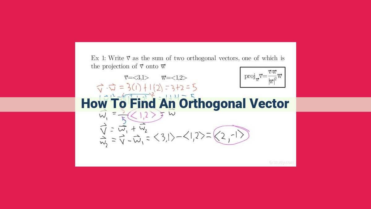
The resulting vector u will be orthogonal to v:

u = w - ((v · w) / |v|^2) * v

Example

Suppose we have a vector v = (2, 3). To find an orthogonal vector to v, let’s choose w = (1, 0):

• Dot product: v · w = (2)(1) + (3)(0) = 2
• Projection of _w_ onto _v_: ((v · w) / |v|^2) * v = ((2) / (2^2 + 3^2)) * (2, 3) = (2 / 13) * (2, 3) = (4/13, 6/13)
• Orthogonal vector _u_: w – ((v · w) / |v|^2) * v = (1, 0) – (4/13, 6/13) = (9/13, -6/13)

Therefore, an orthogonal vector to v = (2, 3) is u = (9/13, -6/13).