Solving Equations With Two Unknowns: Ultimate Guide To Methodologies

Solving equations with two unknowns involves finding values for x and y that satisfy two equations. The substitution method replaces one variable with an expression from another equation, while the elimination method multiplies and adds equations to eliminate one variable. The graphing method plots both equations and finds their intersection point. Matrix method uses matrices and row operations, and Cramer’s Rule employs determinants and matrix inversion. Each method has its advantages, and the most suitable choice depends on the complexity of the system.

• Overview of concepts and different methods for solving systems with two unknowns.

Solving Systems of Linear Equations with Two Unknowns: A Step-by-Step Guide

In the realm of mathematics, solving systems of linear equations with two unknowns is a fundamental skill that unlocks doors to various problem-solving scenarios. Embark on a journey through this blog to grasp the concepts and techniques that will transform you into a linear equation solver extraordinaire.

Meet the Unknowns

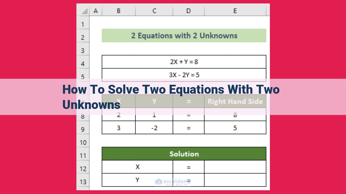
Consider a system of two linear equations with two unknowns, typically represented as x and y. For instance, imagine a grocery store selling apples (x) and oranges (y). To determine how many fruits each variety contributes to a shopper’s purchase, you must solve these equations based on the number of fruits purchased and their respective costs.

Unveiling the Methods

To conquer this algebraic challenge, there’s a palette of methods to choose from, each with its unique strengths. Let’s dive into the most popular techniques:

• Substitution Method: Exchange the role of one unknown for its equivalent expression and solve for the other unknown. Like a magician’s trick, it’s a quick fix if one variable stands out.
• Elimination Method: Pit the equations against each other by multiplying or dividing strategically to eliminate a variable, leaving you with a solitary equation to solve. It’s like playing a game of elimination, where one variable bows out gracefully.
• Graphing Method: Plot the equations as lines on a graph. The point where they intersect, like a celestial harmony, yields the solution. It’s a visual approach that can provide a clear picture.
• Matrix Method: Envision the system as an organized table called an augmented matrix. Perform mathematical operations on its rows to transform it into a simpler form, revealing the solutions like hidden treasures.
• Cramer’s Rule: Unleash the power of determinants, the mathematical gatekeepers of matrices. This rule offers a formulaic approach to solving systems, providing a swift solution if determinants behave kindly.

The Road Ahead

This blog post is your roadmap to mastering systems of linear equations with two unknowns. Each subsequent section will delve into a specific method, guided by examples and problem-solving strategies. As you progress through the chapters, you’ll witness the elegance and versatility of these techniques. So, buckle up, grab a pen and paper, and let’s embark on this algebraic adventure.

The Substitution Method: Unlocking Linear Systems

In the realm of mathematics, solving systems of linear equations is a fundamental skill that empowers us to uncover the intricate relationships between variables. One of the most straightforward and widely used methods for tackling these equations is the substitution method.

Substitution: The Key to Success

The substitution method revolves around the ingenious idea of substituting the expression of one variable into the other equation. By doing so, we effectively eliminate one unknown and reduce the system to a single equation with a single unknown.

Steps to Conquer the Substitution Method:

1. Identify the Equation with a Variable: Inspect the given system of equations and choose the equation that expresses one variable in terms of the other.

2. Substitute the Expression: Plug the identified expression into the remaining equation, replacing all instances of the eliminated variable.

3. Solve for the Remaining Variable: The resulting equation now contains only one unknown. Solve it using your preferred techniques (e.g., factoring, quadratic formula).

Related Concepts: Back and Forward Substitution

The substitution method often paves the way for back substitution or forward substitution. Back substitution involves using the solved value of one variable to find the value of another variable in the original expression. Forward substitution, on the other hand, uses the solved value to find the values of the variables in the eliminated equation.

Connection to Gaussian Elimination

The substitution method shares a deep connection with Gaussian elimination, a more systematic approach for solving linear systems. In fact, substitution can be seen as a simplified version of Gaussian elimination that focuses on eliminating one variable at a time.

Optimizing Your Writing for SEO

To enhance your blog post’s visibility and search engine ranking, consider incorporating relevant keywords such as “solving systems of linear equations,” “substitution method,” “Gaussian elimination,” and “linear algebra.”

Elimination Method: A Step-by-Step Guide

Solving systems of linear equations with two unknowns can be a daunting task, but the Elimination Method provides a straightforward approach to finding solutions efficiently.

The Elimination Method involves manipulating equations to eliminate one variable, allowing you to solve for the remaining variable. This technique shines when dealing with equations where one variable has opposite coefficients, making it easy to combine them out.

Step 1: Equate Coefficients of One Variable

Start by examining your equations. If the coefficients of one variable in both equations are opposites, you’re in luck! For instance, if you have the equations:

3x + 2y = 11
-3x + y = 4

Add the two equations to eliminate the 3x terms:

(3x + 2y) + (-3x + y) = 11 + 4
3y = 15

Step 2: Solve for the Remaining Variable

Now that you’ve eliminated one variable, solve the remaining equation for y:

3y = 15
y = 15 / 3
**y = 5**

Step 3: Substitute and Solve for the Eliminated Variable

Substitute the value of y back into one of the original equations to find the value of x:

3x + 2y = 11
3x + 2(5) = 11
3x + 10 = 11
3x = 11 - 10
**x = 1/3**

Related Concepts:

• Gaussian Elimination: The Elimination Method is essentially a simplified form of Gaussian elimination, a technique for solving systems of equations with multiple variables.
• Row Echelon Form: When using Gaussian elimination, the goal is to transform the original matrix into row echelon form, where the coefficients form a staircase pattern and the system is easier to solve.

Solving Systems of Linear Equations with Two Unknowns: The Graphing Method

In the realm of algebra, systems of linear equations hold a prominent place. These systems, consisting of equations with two or more variables, pose a challenge that requires careful and methodical approaches to unravel their solutions. Among the various methods for solving such systems, the graphing method stands out as a visually intuitive technique that transforms equations into graphs and seeks their intersection as the ultimate solution.

The graphing method is particularly suited for systems of two linear equations, where each equation represents a straight line in a two-dimensional plane. To embark on this method, we begin by isolating each equation in slope-intercept form:

y = mx + b

In this form, m and b represent the slope and y-intercept of the line, respectively. Once we have our equations in this format, we can effortlessly graph them on a coordinate plane. The coordinates of the point where these lines intersect provide the solution to our system of equations.

However, it’s important to note that there can be three possible outcomes when graphing systems of linear equations:

• One intersection point: This occurs when the lines intersect at a single point, indicating a unique solution.
• Infinitely many intersection points: This happens when the lines coincide, forming a single line. In this case, there are an infinite number of solutions.
• No intersection points: This occurs when the lines are parallel and never meet. In this case, there is no solution.

To enhance the accuracy of our solution, it’s advisable to graph the lines on graph paper or utilize graphing software. This visual representation makes it easier to identify the intersection point and determine the solution.

The graphing method is particularly useful when we want to visualize the relationship between the variables and the solution. It provides a graphical understanding of the system, making it an effective tool for learners and educators alike.

The Matrix Method: A Powerful Tool for Solving Systems of Linear Equations

Imagine you’re a detective tasked with solving a cryptic puzzle. The puzzle is a system of linear equations with two unknowns, like a tangled web of clues. To unravel this enigma, you’ll need a technique that’s both precise and efficient—the Matrix Method. It’s time to don your detective hat and embark on the thrilling journey of solving systems with this powerful tool.

Step 1: The Augmented Matrix

The first step is to transform our system of equations into an augmented matrix. This matrix is a rectangular array of numbers that contains both the coefficients of the variables and the constants. By organizing our equations in this way, we create a visual representation of the system that makes it easier to manipulate.

Step 2: Row Operations

Once we have our augmented matrix, it’s time for the magic to begin. We’ll perform a series of row operations to transform the matrix into a form that’s easier to solve. These operations include:

• Swapping rows: Rearranging the order of rows to simplify the matrix.
• Multiplying a row by a constant: Scaling a row to make its elements more manageable.
• Adding or subtracting a multiple of one row to another: Combining rows to eliminate variables.

Step 3: Row Echelon Form

Through these row operations, we aim to achieve row echelon form. This is a special form of the matrix where the leading coefficient (the leftmost non-zero element) of each row is 1 and all other elements in that column are 0. Once our matrix is in row echelon form, solving for the variables becomes a simple matter of back-substitution.

Step 4: Back-Substitution

Starting with the bottom row, we can solve for the last variable because it only appears in one equation. Once we have its value, we can substitute it back into the previous row to solve for the next variable, and so on. This process of back-substitution allows us to find the values of all the variables in a systematic and efficient manner.

The Matrix Method is not just another technique for solving systems of linear equations—it’s an invaluable tool that transforms complex problems into solvable ones. By representing the system as an augmented matrix and performing row operations, we can simplify the system, eliminate variables, and ultimately find the solutions with ease. So next time you encounter a system of linear equations, remember the Matrix Method—your trusty companion on the path to solving complex puzzles.

Cramer’s Rule: A Formulaic Approach to Solving Systems of Equations

Cramer’s Rule, a powerful tool in linear algebra, offers a systematic approach for solving systems of linear equations with two unknowns. It replaces the need for intricate algebraic manipulations.

Definition and Steps

Cramer’s Rule employs determinants to compute the values of variables in a system. For a system of equations:

a₁x + b₁y = c₁
a₂x + b₂y = c₂

Let’s denote the determinant of the coefficients as:

D = |a₁  b₁|
    |a₂  b₂|

The value of x is then calculated as:

x = (|c₁  b₁|) / D

Similarly, the value of y is determined as:

y = (|a₁  c₁|) / D

Related Concepts

Determinants are numerical values derived from square matrices, providing insights into the relationships between the matrix’s rows and columns. Matrix inversion, another crucial concept, involves finding the inverse matrix of a given square matrix. This inverse matrix, when multiplied by the original matrix, results in the identity matrix.

Advantages and Limitations

Cramer’s Rule shines in solving systems with low-order matrices, typically 2×2 or 3×3 matrices. However, it becomes computationally intensive for larger matrices. Furthermore, the method is not applicable to systems with dependent equations or when the determinant of the coefficients matrix is zero.

Example

For the system:

2x - 3y = 1
x + 2y = 5

Determinant of the Coefficients:

|2  -3|
|1   2| = 7

Solving for x:

x = (|1  -3|) / 7 = 4 / 7

Solving for y:

y = (|2   1|) / 7 = 3 / 7

Thus, the solution to the system is (x, y) = (4/7, 3/7).

Cramer’s Rule provides a straightforward approach for solving systems of linear equations when the order of the coefficient matrix is small. Its reliance on determinants allows for efficient computation of variable values. However, for larger systems or those with dependent equations, other methods, such as Gaussian elimination, may be more suitable.