Uncover Quadratic Equations With Precision: A Comprehensive Guide
From a table, plot data points and calculate differences to uncover a quadratic equation in the form y = Ax^2 + Bx + C. Determine the second difference of y-coordinates to find the coefficient A. Substitute a point to solve for B and C. This method enables you to model data with a quadratic equation, facilitating analysis and problem-solving in various fields.
Finding Quadratic Equations from Tables: Unlocking the Secrets of Curves
Are you ready to embark on a journey where numbers dance in perfect harmony, forming curves that reveal hidden secrets? Join us as we delve into the world of quadratic equations and unveil the intriguing art of finding them from a simple table.
Why Quadratic Equations Matter?
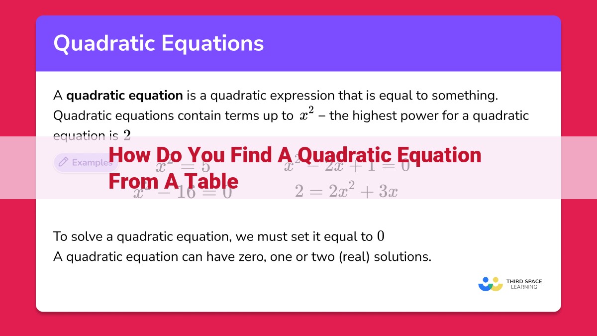
These equations are like the masters of curves, shaping everything from parabolic paths to the growth patterns of bacteria. They have their hands in physics, engineering, economics, and countless other fields, making them essential tools for understanding the world around us.
Unveiling the Table’s Story
Imagine a table with a series of numbers, each representing a hidden equation. Our goal is to decipher that equation, revealing the curve that connects the dots. The first step is to plot the points on a graph, creating a visual representation of our data. This allows us to see patterns and trends that might otherwise be hidden.
Next, we embark on a journey of calculating differences, comparing the x and y coordinates of our points. These differences hold the key to unraveling the equation. Specifically, the second difference of the y-coordinates will guide us towards the coefficient of the quadratic term (Ax^2).
Writing the Quadratic Equation
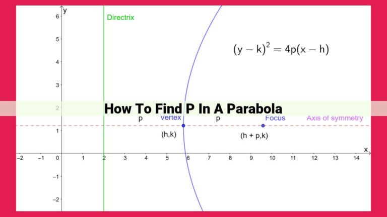
Armed with the second difference, we can now start assembling our equation. We begin with the standard form: y = Ax^2 + Bx + C. Substituting the second difference into the formula, we solve for the coefficient A, determining the shape of our curve.
Fitting the Pieces Together
To find the remaining coefficients, B and C, we employ a clever trick. We choose a data point from the table and substitute its coordinates into our equation. This allows us to create a system of equations, which we can then solve to find B and C.
Example: Unveiling the Hidden Curve
Let’s consider a table with the following data:
| x | y |
|---|---|
| 1 | 2 |
| 2 | 6 |
| 3 | 12 |
Following the steps outlined above, we can find the quadratic equation that fits this data:
y = 2x^2 + 2x + 2
And there you have it, the secrets of finding quadratic equations from tables revealed. By understanding the underlying patterns and relationships between the data points, we can unlock the equations that govern the curves that surround us. From understanding parabolic trajectories to predicting growth rates, quadratic equations are an invaluable tool in our quest to make sense of the world. So, next time you encounter a table of numbers, remember the techniques you’ve learned and embark on a journey of discovery, uncovering the hidden equations that shape our world.
Plotting the Points: A Journey of Visualization and Discovery
In the quest to uncover the elusive quadratic equation hidden within a mysterious table of data, plotting the points is a crucial step, a cartographer’s art that transforms raw numbers into a visual landscape.
Each point, a small beacon of information, is meticulously placed on the graph, like a pin marking a location on a map. The X-axis, like an unyielding ruler, measures the march of the independent variable, while the Y-axis, a celestial guide, tracks the changes in the dependent variable.
As the points take their places, a mosaic of data emerges before our eyes, a tapestry woven with the threads of observation. We can now see the shape of the relationship between the variables, its highs and lows, its twists and turns.
Plotting points is not merely a mechanical exercise; it’s an invitation to explore. By visualizing the data, we gain a deeper understanding of its patterns, its anomalies, and its potential secrets. It’s the first step towards unlocking the enigmatic code of the quadratic equation.
Calculating Differences:
- Describe how to calculate the differences between the x-coordinates and y-coordinates.
- Explain the significance of these differences in determining the quadratic equation.
Calculating Differences: Delving into the Essence of Quadratic Equations
In the realm of mathematics, quadratic equations hold a prominent position, serving as fundamental tools in modeling real-world phenomena. They enable us to describe relationships that exhibit parabolic patterns, such as the trajectory of a projectile or the growth of a population over time. To unravel the mysteries of these equations, we embark on a journey of discovery, beginning with a crucial step: calculating differences.
X-coordinate Differences: Unveiling the Underlying Structure
Consider a table of values that represents a quadratic equation. The first step in our quest is to calculate the differences between the x-coordinates of consecutive data points. These differences, denoted as ‘Δx’, provide valuable insights into the equation’s underlying structure.
Y-coordinate Differences: A Stepping Stone to Discovery
Next, we turn our attention to the y-coordinates. The second step involves calculating the differences between the y-coordinate differences. These second-order differences, denoted as ‘Δ²y’, hold the key to unlocking the quadratic equation’s coefficient of the x² term (Ax²).
Significance of Differences: A Guiding Light in the Equation’s Landscape
The significance of these differences lies in their ability to reveal the equation’s characteristics. The Δx values establish the spacing between points on the x-axis, while the Δ²y values provide a measure of the curve’s curvature. By carefully analyzing these differences, we gain valuable clues about the equation’s shape and behavior.
Armed with these calculated differences, we forge ahead to the next step in our equation-solving adventure: finding the second difference of the y-coordinates. Stay tuned as we delve deeper into this journey of mathematical discovery!
Finding the Second Difference of Y-coordinates:
- Provide the formula for calculating the second difference between the y-coordinate differences.
- Emphasize the importance of this step in determining the coefficient of the quadratic term (Ax^2).
Finding the Second Difference of Y-Coordinates: The Key to Unlocking Quadratic Equations
As we delve deeper into our journey of extracting quadratic equations from tables, we reach a crucial juncture that holds the key to unraveling the equation’s hidden coefficients: calculating the second difference of the y-coordinates. This step forms the cornerstone for determining the coefficient of the quadratic term (Ax²) and sets the stage for completing the equation.
The second difference is calculated by subtracting the subsequent differences between the consecutive y-coordinates. In simpler terms, we take the difference of the differences between the y-values. This seemingly simple operation reveals a profound pattern that holds the secret to the quadratic equation.
For instance, let’s consider a table with y-coordinates: [2, 6, 12, 20]. The differences between these values are [4, 6, 8]. The next step is to calculate the second difference, which is the difference between the differences: 6 – 4 = 2. This number, the second difference, is of paramount importance in uncovering the coefficient of the quadratic term in the equation.
Its significance lies in the fact that the second difference corresponds directly to the coefficient of the quadratic term (Ax²). By establishing this connection, we pave the way for completing the quadratic equation and understanding its behavior.
Determining the Quadratic Equation: Unveiling the Key Terms
In the realm of mathematics, quadratic equations hold immense significance, providing a potent tool for modeling a wide range of real-world phenomena. These equations find applications in fields spanning physics, engineering, and economics. To harness the power of quadratic equations, we embark on a journey to derive them from a tabular representation of data.
A quadratic equation takes the form of y = Ax² + Bx + C, where A, B, and C are constants. Our quest begins with A, the coefficient of the quadratic term.
To determine the value of A, we must delve into the concept of second difference. The second difference is the difference between consecutive differences between adjacent values in a data set. In the context of a table of values representing a quadratic function, the second difference of the y-coordinates remains constant and is numerically equal to 2A.
Unveiling the Value of A
With this newfound understanding, we can substitute the second difference into the formula A = 2nd difference / 2. This elegant equation provides us with the key to unlocking the value of A.
Determining the Coefficients B and C
In the journey to uncover the enigmatic quadratic equation hidden within a table of data, we have meticulously calculated the second difference of the y-coordinates, revealing the elusive coefficient A. However, our quest is far from over, as we must now unravel the secrets of the remaining coefficients, B and C.
Enter the technique of substitution, a powerful tool that allows us to extract these coefficients from the depths of the table. Like a skilled detective, we will select one data point from our table and plug its coordinates (x, y) into our newly discovered quadratic equation:
y = Ax² + Bx + C
By doing so, we create an equation that holds a treasure trove of information. Solving this equation grants us the power to determine the values of B and C, the elusive coefficients that shape our quadratic equation.
Consider a specific data point (x₁, y₁). Substituting its coordinates into the quadratic equation, we obtain:
y₁ = Ax₁² + Bx₁ + C
This equation holds the key to unlocking the secrets of B and C. Using algebra, we can rearrange it to isolate B and C:
B = (y₁ - Ax₁²) / x₁
C = y₁ - Ax₁² - Bx₁
With these formulas, we have forged the tools to solve for B and C. By substituting the known values of x₁, y₁, and A into these formulas, we can illuminate the true nature of our quadratic equation.
Thus, the enigmatic coefficients B and C, once shrouded in mystery, are now revealed, breathing life into the quadratic equation that captures the essence of the data before us.
Unveiling the Quadratic Equation from a Table: A Step-by-Step Guide
In the captivating realm of mathematics, quadratic equations play a crucial role in modeling real-world scenarios from projectile motion to optimizing business strategies. To uncover the elusive quadratic equation hiding within a data table, embark on this step-by-step journey filled with mystery and intrigue.
Plotting the Puzzle Pieces (Plotting the Points)
Like a treasure hunter marking an ancient map, carefully plot the given points from the data table onto a graph. Each point represents a clue leading to the unknown quadratic equation. The resulting scatterplot paints a visual tableau, providing insights into the underlying pattern.
Unraveling the Patterns (Calculating Differences)
With meticulous precision, delve into the depths of the table, unveiling the differences between the x-coordinates and y-coordinates. These differences, like threads in a tapestry, intertwine to reveal the intricate design of the quadratic equation.
The Gateway to Discovery (Finding the Second Difference of Y-coordinates)
Venture into the labyrinth of y-coordinate differences and unearth their hidden secrets. Calculate the second difference between them, akin to a beacon illuminating the path towards the coefficient of the quadratic term (Ax^2).
Craft the Quadratic Masterpiece (Writing the Quadratic Equation)
Harnessing the power of the second difference, substitute its value into the hallowed halls of the standard quadratic equation (y = Ax^2 + Bx + C). Behold as the coefficient of the quadratic term takes shape, revealing a piece of the enigmatic puzzle.
Solving for the Unknown (Substituting a Point)
Like a master detective scrutinizing a crime scene, select a data point from the table and substitute its coordinates into the quadratic equation. Engage in the art of solving for B and C, using substitution and the elegance of a system of equations.
A Guiding Light in the Mathematical Labyrinth (Example)
To illuminate the path ahead, consider the following data table:
| x | y |
|---|---|
| 0 | 2 |
| 1 | 5 |
| 2 | 10 |
Embark on the captivating journey of finding the quadratic equation that governs these data points:
- Plot the points on a graph to create a visual representation.
- Calculate the differences between the x-coordinates and y-coordinates: 1, 5.
- Determine the second difference of the y-coordinate differences: 4.
- Substitute the second difference into the standard quadratic equation: y = 4x^2 + Bx + C.
- Select a data point (0, 2) and substitute its coordinates into the equation: 2 = 40^2 + B0 + C.
- Solve for B: 2 = C.
- Substitute C = 2 back into the quadratic equation: y = 4x^2 + Bx + 2.
- Substitute the other data point (1, 5) into the equation: 5 = 41^2 + B1 + 2.
- Solve for B: 3 = B.
- The quadratic equation is y = 4x^2 + 3x + 2.
Through the intricate steps of plotting, calculating, and solving, we have successfully unraveled the quadratic equation that governs the given data table. This equation serves as a powerful tool for understanding and predicting the relationship between the variables in real-world scenarios, empowering us to make informed decisions and solve complex problems.