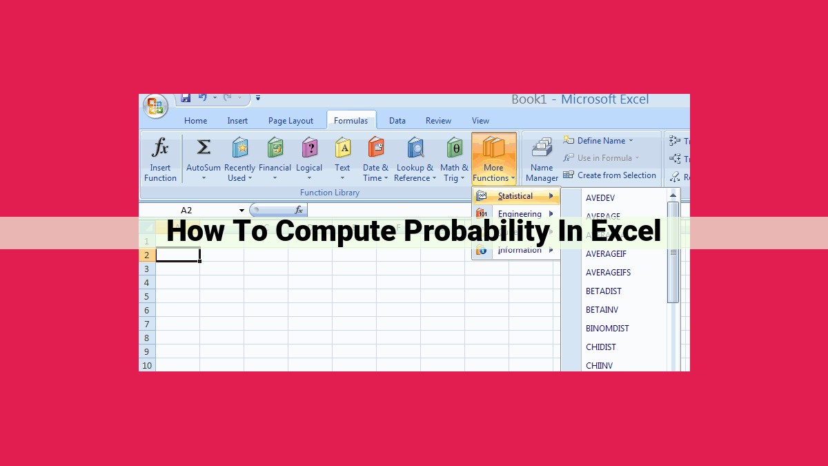
Excel Functions For Probability Calculations: A Comprehensive Guide

Excel provides robust functions for calculating probabilities in various scenarios. The RAND function generates random numbers between 0 and 1, while RANDBETWEEN produces random integers within a range. NORMINV calculates probabilities under the normal distribution, BINOMDIST models binomial processes, POISSON computes probabilities of randomly occurring events, and CHIINV, TINV, and FINV convert probabilities to critical values for chi-square, t-tests, and F-tests, respectively. These functions enable efficient and accurate probability calculations for simulations, sampling, and statistical analyses.

Unlocking the Power of Excel Functions for Probability Calculations: A Game-Changer for Data Analysis

In the realm of data analysis, probability plays a pivotal role in understanding the likelihood of events and making informed decisions. Excel, the ubiquitous spreadsheet software, empowers you with a suite of powerful functions that can effortlessly perform complex probability calculations, opening up a world of possibilities for your data analysis endeavors.

Excel’s probability functions are invaluable tools for various industries, from finance to healthcare, empowering professionals to delve deeper into their data and unravel hidden insights. Whether you’re an expert in statistics or just starting your journey, this guide will equip you with the knowledge and confidence to harness the power of Excel’s probability functions.

Navigating the Excel Probability Functions Landscape

Excel offers a comprehensive array of probability functions, each tailored to specific calculations. From generating random numbers and simulating events to calculating probabilities under various distributions, these functions provide a versatile toolkit for your data analysis needs.

Unleashing the Power of Excel’s RAND Function for Probability Calculations

In the realm of probability, Excel’s RAND function stands as a formidable tool. It allows you to generate random numbers between 0 and 1, opening up a world of possibilities for simulations and random sampling.

How RAND Works:

RAND, when entered into a cell, produces a random number between 0 (inclusive) and 1 (exclusive). Each time you enter or recalculate the function, you get a different number, ensuring true randomness.

Applications in Simulations:

Simulations are essential for modeling complex systems and predicting outcomes. By generating random numbers, RAND enables you to mimic real-world scenarios and perform repeated trials. For example, you can simulate coin flips, dice rolls, or more sophisticated scenarios like customer behavior or disease spread.

Random Sampling Techniques:

RAND also finds its use in random sampling techniques. By generating a random sample of data, you can obtain a representative subset that reflects the larger population. This method is crucial for statistical analysis, survey research, and quality control.

Additional Tips:

• To generate a random integer within a specified range, use the RANDBETWEEN function.
• To ensure that the random numbers are not tied to your computer’s clock, turn off automatic recalculation in Excel’s Options.
• Use volatile functions (e.g., NOW()) alongside RAND to create dynamic simulations that change with time.

Mastering the RAND function in Excel empowers you to explore the world of probability with ease and confidence. Its versatility and simplicity make it an invaluable tool for researchers, analysts, and anyone looking to harness randomness for their projects.

Unlocking the Power of Probability with the RANDBETWEEN Function

In the realm of data analysis, Excel’s probability functions provide a powerful tool for calculating the likelihood of events and predicting outcomes. Among these functions, the RANDBETWEEN function stands out as a versatile tool for generating random integers within a specified range.

Generating Random Integers Made Easy

The RANDBETWEEN function takes two arguments: the lower and upper bounds of the range. It returns a random integer that falls within this range, inclusive. This function is particularly useful when you need to select elements or values at random, such as:

• Randomly selecting participants for a survey
• Simulating the roll of dice in a game
• Generating unique lottery numbers

Simulating Chance Encounters

The RANDBETWEEN function also excels in creating realistic simulations. For instance, if you’re modeling a product defect rate, you can use the function to generate random integers representing the number of defective products within a specified batch. This allows you to estimate the probability of encountering a defective product.

Adding a Touch of Luck to Lottery Simulations

Lottery simulations are another exciting application of the RANDBETWEEN function. By generating random integers within a specific range, you can create a realistic representation of a lottery draw. This can be used to analyze the probability of winning, experiment with different strategies, or simply provide a fun and interactive way to simulate the thrill of a lottery draw.

The RANDBETWEEN function is an indispensable tool for a wide range of probability calculations and simulations. Its ability to generate random integers within a specified range makes it perfect for tasks such as selecting random elements, creating realistic models, and even designing lottery simulations. As you explore the depths of probability with Excel, don’t forget the power of this versatile function.

Delving into the Secrets of NORMINV: Unlocking Probability’s Mysteries

In the vast realm of probability and statistics, the normal distribution holds a place of great significance. It governs a myriad of real-world phenomena, from heights of individuals to exam scores. Understanding its nuances is crucial for making informed decisions and drawing meaningful conclusions.

The NORMINV function is an Excel workhorse that empowers you to navigate the intricacies of the normal distribution with ease. This function bridges the gap between z-scores and probabilities. A z-score measures the distance of a data point from the mean in units of standard deviations.

By harnessing the NORMINV function, you can convert z-scores into their corresponding probabilities. This conversion unveils the likelihood of an event falling within a particular range of the normal distribution. For example, you can ascertain the probability of a student scoring between 68% and 95% on a standardized test, given that the mean score is 80% and the standard deviation is 10%.

Furthermore, the NORMINV function provides insights into the deviation from the mean. You can specify the desired level of deviation (in terms of z-scores) and determine the probability of an event occurring within that range. This empowers you to make informed decisions based on the likelihood of various outcomes.

To use the NORMINV function in Excel, simply follow these steps:

1. Select an empty cell where you want to display the probability.
2. Type the formula “=NORMINV(z-score, mean, standard_deviation)”
3. Replace “z-score” with the desired z-score.
4. Replace “mean” with the mean of the normal distribution.
5. Replace “standard_deviation” with the standard deviation of the normal distribution.

Unlock the secrets of the normal distribution with the NORMINV function. It empowers you to convert z-scores to probabilities and explore deviations from the mean, empowering you to make informed decisions and unravel the mysteries of probability.

Unlocking the Power of Excel for Binomial Probability Calculations

In the realm of probability, there’s a treasure trove of functions waiting to be harnessed in Excel, and the BINOMDIST function shines as a formidable tool for understanding and modeling binomial processes.

Imagine you’re flipping a coin, trying to predict the probability of landing on heads n times in a row. Or perhaps you’re analyzing manufacturing data, estimating the likelihood of defective products within a batch. The BINOMDIST function becomes your trusty companion in these scenarios.

What’s a Binomial Process?

A binomial process is a sequence of independent trials where each trial has only two possible outcomes. For instance, flipping a coin (heads or tails) or checking for product defects (defective or not defective) are classic examples.

Using the BINOMDIST Function

The BINOMDIST function takes four arguments:

1. number_s: The number of successes you want to calculate the probability for.
2. trials: The total number of trials.
3. probability_s: The probability of success on each trial.
4. cumulative: A logical value (TRUE or FALSE) that specifies whether to return the cumulative probability or just the probability for the specified number of successes.

Example: Coin Toss Simulation

Let’s say you want to find the probability of flipping heads exactly three times in a row. Using the BINOMDIST function, you can enter:

=BINOMDIST(3, 5, 0.5, FALSE)

where:

• number_s = 3 (flips with heads)
• trials = 5 (total flips)
• probability_s = 0.5 (probability of heads on each flip)
• cumulative = FALSE (return the probability for exactly three heads)

This formula will output the probability of getting exactly three heads, which in this case is 0.3125.

Modeling Binomial Processes

The BINOMDIST function is also invaluable for modeling binomial processes. For instance, if you’re curious about the probability of finding at least one defective product in a batch of 100 items, where the defect rate is known to be 5%, you can use the BINOMDIST function to calculate it.

Mastering the BINOMDIST function unlocks a world of possibilities for probability calculations and binomial process modeling. Whether you’re analyzing coin tosses, manufacturing data, or any other scenario that involves two possible outcomes, this function empowers you to harness the power of probability in Excel.

Unlocking the Power of Probability Calculations with Excel’s Poisson Function

The Poisson Distribution: A Guiding Light for Random Occurrences

Picture this: You’re analyzing the number of phone calls received by a customer service center each hour. How do you predict the likelihood of receiving a specific number of calls? Enter the Poisson distribution, a mathematical tool that models events occurring randomly within a fixed interval.

Excel’s POISSON Function: A Master Mathematician

Microsoft Excel’s POISSON function is your go-to tool for calculating Poisson probabilities. It takes two arguments: lambda and x. Lambda represents the average number of occurrences expected within the interval, while x specifies the actual number of occurrences you’re interested in.

Unveiling the Probability Riddle

Suppose you want to determine the probability of receiving exactly 5 phone calls within the next hour, assuming an average of 3 calls per hour. Plug the values into the POISSON function:

POISSON(3, 5)

This formula yields a probability of 0.1353. In other words, there’s a 13.53% chance of receiving precisely 5 calls within that hour.

Real-World Applications: Embracing the Poisson

The POISSON function is an invaluable tool in various fields:

• Customer Service: Predicting call volumes and staffing needs
• Manufacturing: Modeling product defects and setting quality control parameters
• Epidemiology: Estimating disease incidence and outbreak risks
• Finance: Calculating insurance premiums and investment risk assessments

Unlocking the Secret of Poisson Probabilities

Mastering the POISSON function empowers you to make informed decisions based on probability calculations. By understanding the Poisson distribution and leveraging Excel’s mathematical prowess, you can confidently navigate the world of random occurrences and unravel the mysteries of probability.

Leveraging the CHIINV Function: A Guide to Probability and Statistical Calculations in Excel

In the realm of probability and statistics, the chi-square distribution plays a crucial role in hypothesis testing. And to navigate this distribution effectively, the CHIINV function in Excel becomes an indispensable tool.

Unlocking the Chi-Square Universe with CHIINV

The CHIINV function is designed to convert a specified probability value under the chi-square distribution to its corresponding chi-square value. This conversion is vital for determining critical values in chi-square tests.

Unveiling Chi-Square Critical Values

Chi-square tests evaluate the goodness of fit between observed and expected data. To determine if there’s a significant difference between these values, we need to establish critical values. The CHIINV function helps us find these critical values at a specified significance level.

By setting the probability argument in the CHIINV function to the appropriate significance level (e.g., 0.05 for a 5% significance level) and specifying the degrees of freedom for the chi-square distribution, we can obtain the critical chi-square value.

Practical Applications of CHIINV

The CHIINV function finds widespread use in statistical applications, including:

• Identifying outliers in a dataset by comparing the observed chi-square value to the critical chi-square value.
• Testing the independence of two categorical variables by comparing the observed chi-square value to the critical value for a specified significance level.
• Determining the goodness of fit between a sample and a theoretical distribution by calculating the chi-square statistic and comparing it to the critical value.

Embracing the Power of CHIINV

Mastering the CHIINV function empowers you to navigate the complexities of probability and statistical calculations with ease. By harnessing its capabilities, you can confidently delve into hypothesis testing, determine critical values, and make informed decisions based on statistical evidence.

Using the TINV Function

• Converting t-probabilities to t-values
• Calculating critical values for t-tests

Using the TINV Function in Excel for Probability Calculations

In the vast realm of probability, the TINV function wields its power as a pivotal tool for statisticians, data analysts, and anyone seeking to unravel the intricacies of t-distributions. Understanding its nuances not only empowers us with precise probability calculations but also paves the way for conducting accurate hypothesis tests.

The TINV function in Excel converts t-probabilities into t-values, enabling us to determine critical values for t-tests. A t-test is a statistical test used to compare the means of two independent groups, providing valuable insights into whether there is a significant difference between the two populations they represent.

To harness the potential of the TINV function, we must delve into the concept of t-distributions. These distributions are bell-shaped and resemble normal distributions, but their tails are heavier, indicating a greater likelihood of extreme values. The degree of freedom parameter in a t-distribution influences its shape and behavior.

To calculate a critical value for a t-test using the TINV function, we need the probability, the degrees of freedom, and the tail type (one-tailed or two-tailed test). The probability represents the area under the t-distribution curve beyond the critical value. The degrees of freedom determine the shape of the t-distribution, and the tail type specifies whether we are interested in only one tail or both tails of the distribution.

For instance, if we wish to test whether the mean height of students in two different schools is significantly different, we can calculate the critical values using the TINV function. By setting the probability to 0.05 (assuming a 95% confidence level) and the degrees of freedom to the total sample size minus 2 (assuming independent samples), we obtain the critical values that serve as the boundaries for rejection regions in our hypothesis test.

Mastering the TINV function allows us to interpret t-test results with precision, helping us make informed decisions based on statistical evidence. It opens doors to a deeper understanding of probability distributions, hypothesis testing, and the power of Excel in empowering data analysis.

Unveiling the Secrets of the FINV Function: A Guide to F-Probabilities and Critical Values

In the realm of Excel functions, the FINV function stands as a gatekeeper to the mysteries of F-distributions. It unveils the hidden connections between probabilities and F-values, empowering you with the ability to decipher the outcomes of F-tests.

Unlocking the Power of F-Probabilities

Just as a coin determines the probability of getting heads or tails, the F-distribution determines the probability of obtaining a particular F-statistic in a statistical test. The FINV function serves as a trusty translator, converting these probabilities into their corresponding F-values. This knowledge grants you the power to set thresholds for your F-test, ensuring that you make informed decisions about rejecting or accepting the null hypothesis.

Conjuring Critical Values for F-tests

The FINV function also plays a pivotal role in calculating critical values for F-tests. These values, like guardian angels, protect the integrity of your statistical analysis. By defining the boundaries of statistical significance, they guide you towards sound conclusions. Whether you’re delving into an ANOVA or a regression analysis, the FINV function provides the blueprint for establishing these critical thresholds.

A Practical Guide to Using FINV

Harnessing the power of the FINV function is a straightforward endeavor. Simply plug in your desired probability, the degrees of freedom for the numerator and denominator, and Excel will reveal the corresponding F-value. For instance, if you’re running an F-test with 5 degrees of freedom in the numerator and 10 degrees of freedom in the denominator, and you want to know the critical value for a significance level of 0.05, the formula would be:

=FINV(0.05, 5, 10)

Excel would then return the F-value of 4.96.

The FINV function is an invaluable tool for anyone navigating the statistical landscape. By unlocking the secrets of F-probabilities and critical values, it empowers you to conduct rigorous F-tests and draw informed conclusions. So, embrace the power of this statistical wizard and conquer the challenges of your next F-test with confidence.