Unlocking Polynomial Functions: End Behavior, Symmetry, And Remainder Theorem

To determine the end behavior of a polynomial, consider its leading coefficient: positive for increasing end behavior, negative for decreasing. The leading coefficient and degree determine the shape of the graph. The test for even and odd functions reveals symmetry. The remainder theorem helps find the remainder when dividing by a linear factor. Factor theorem finds factors. These concepts interconnect to analyze the graph’s end behavior, providing valuable insights for understanding polynomial functions.

Unlocking the Secrets of Polynomial End Behavior: A Guide to Polynomial Analysis

In the realm of mathematics, polynomials stand as the building blocks of complex functions, shaping our understanding of the world around us. Determining the end behavior of a polynomial is a crucial step in unraveling its secrets, providing us with insights into its shape, symmetry, and overall characteristics. Knowing this behavior allows us to make informed predictions about the polynomial’s graph, enabling us to solve equations, analyze functions, and delve into the fascinating world of algebra.

Why is it Important to Understand End Behavior?

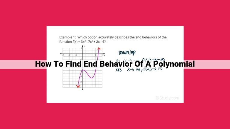
The end behavior of a polynomial reveals its asymptotic tendencies—how the function behaves as its input approaches infinity or negative infinity. This knowledge plays a pivotal role in understanding the overall shape of a polynomial’s graph, helping us identify its important features such as its intercepts, local extrema, and points of inflection. By analyzing the end behavior, we can quickly determine if the function increases or decreases without performing extensive calculations.

Moreover, understanding end behavior is essential for solving equations involving polynomials. By identifying the end behavior of a polynomial expression, we can eliminate potential solutions and narrow down the search for valid roots. This technique significantly streamlines the equation-solving process, saving us time and effort.

Key Concepts for Determining End Behavior

Determining the end behavior of a polynomial involves a combination of key concepts, each providing a unique perspective on the function’s behavior.

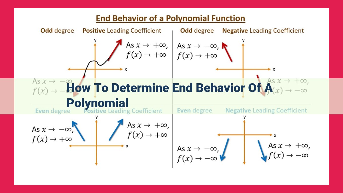
1. Leading Coefficient Test: The leading coefficient, the coefficient of the highest-degree term, determines the overall direction of the polynomial’s end behavior. A positive leading coefficient indicates that the polynomial increases as the input approaches infinity, while a negative leading coefficient indicates a decrease.

2. Test for Even and Odd Functions: This test distinguishes between even and odd functions. An even function exhibits symmetry around the y-axis, while an odd function shows symmetry around the origin. Understanding the symmetry of a polynomial can provide valuable insights into its end behavior, as it helps us determine the function’s behavior at specific points.

3. Degree of the Polynomial: The degree of a polynomial, the highest exponent of the variable, influences the steepness of the polynomial’s end behavior. Higher-degree polynomials generally exhibit more extreme end behavior, increasing or decreasing more rapidly than lower-degree polynomials.

4. Remainder Theorem: The Remainder Theorem tells us the remainder when dividing a polynomial by a linear factor of the form (x – c). This theorem allows us to investigate the end behavior of a polynomial by evaluating it at a specific point, providing valuable information about its behavior near that point.

5. Factor Theorem: The Factor Theorem determines whether a polynomial has a specific factor of the form (x – c). This theorem helps us identify potential roots and factors, which can provide additional insights into the end behavior of the polynomial.

In conclusion, understanding the end behavior of a polynomial is a fundamental concept in polynomial analysis. By combining key concepts such as the leading coefficient test, the test for even and odd functions, the degree of the polynomial, the Remainder Theorem, and the Factor Theorem, we can unlock the secrets of polynomial behavior, enabling us to make informed predictions about their graphs and solve equations with greater efficiency.

Leading Coefficient Test

• Explain how the leading coefficient determines the end behavior.

The Leading Coefficient Test: A Guide to Unlocking Polynomial End Behavior

Polynomials, those enigmatic mathematical expressions that haunt the dreams of students and mathematicians alike, possess a hidden secret that reveals their true nature. Understanding the end behavior of a polynomial, how it behaves as it stretches out towards infinity, is like unlocking a treasure chest of insights into its character.

Among the many tools at our disposal for divining the end behavior of a polynomial, the leading coefficient test stands out as a beacon of simplicity and elegance. This test revolves around a single but crucial piece of information: the coefficient of the term with the highest exponent.

Imagine a polynomial like a roller coaster, its graph snaking its way through the mathematical landscape. The leading coefficient acts like an invisible force, dictating the coaster’s ultimate fate. If the leading coefficient is positive, the coaster will soar towards infinity as it stretches to the right and left. Like an unstoppable force, the polynomial ascends without bound.

Conversely, if the leading coefficient is negative, the coaster will plummet towards negative infinity, its graph spiraling downward as it approaches the ends of the number line. In this case, the polynomial descends into the depths, forever falling away.

The leading coefficient test is a powerful tool for quickly determining the asymptotic behavior of a polynomial. Whether it rises or falls, this test provides a blueprint for understanding the polynomial’s long-term tendencies. So next time you’re confronted with a polynomial enigma, embrace the simplicity of the leading coefficient test and unravel its secrets with newfound confidence.

Test for Even and Odd Functions: Unraveling the Symmetry of Polynomials

In the realm of polynomials, understanding their end behavior is crucial for analyzing their graphs. Among the various tests used to determine this behavior, the Test for Even and Odd Functions plays a significant role in revealing the symmetry of these mathematical expressions.

A polynomial is considered even if it satisfies the even function condition: f(-x) = f(x). This means that the graph of an even function is symmetrical about the y-axis. In other words, if you fold the graph along the y-axis, the two halves will coincide.

On the other hand, a polynomial is considered odd if it meets the odd function condition: f(-x) = -f(x). In this case, the graph of an odd function is symmetrical about the origin. If you rotate the graph 180 degrees around the origin, it will coincide with itself.

Determining Even and Odd Functions

To determine whether a polynomial is even or odd, simply plug in -x for x in the original expression. If the resulting expression is the same as the original, the polynomial is even. If it is the negative of the original, the polynomial is odd.

Examples

Consider the polynomial f(x) = x^2 – 4. Substituting -x for x gives f(-x) = (-x)^2 – 4 = x^2 – 4, which is the same as f(x). Therefore, f(x) is an even function, and its graph is symmetrical about the y-axis.

Now, let’s examine g(x) = x^3 – 2x. Plugging in -x yields g(-x) = (-x)^3 – 2(-x) = -x^3 + 2x, which is the negative of g(x). Hence, g(x) is an odd function, and its graph is symmetrical about the origin.

Understanding the even or odd nature of a polynomial is vital for analyzing its graph and understanding its symmetries and behaviors at infinity. By applying the Test for Even and Odd Functions, we can gain valuable insights into the shape and characteristics of these mathematical expressions.

The Degree of Polynomial: Shaping the Graph’s Landscape

When exploring polynomial graphs, the degree takes center stage, influencing their shape like a maestro orchestrating a symphony. The degree, measured as the highest exponent of the variable, dictates the polynomial’s overall curvature and complexity.

Consider a linear function with a degree of 1. Its graph is a straight line that steadily increases or decreases, forming a simple, linear pattern. As the degree increases, the graph takes on a more dramatic shape.

A quadratic function of degree 2 boasts a parabolic curve, rising and falling gracefully like a roller coaster. The curve’s concavity, whether upward or downward, depends on the coefficient of the squared term.

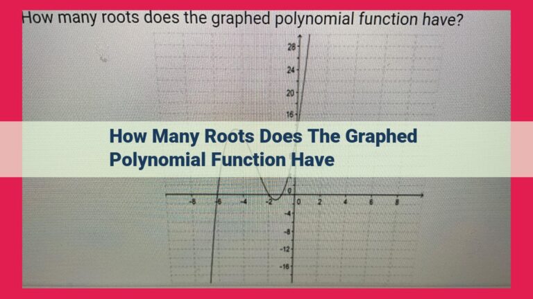
For polynomials with degrees higher than 2, the graph acquires multiple turning points and becomes more intricate. Cubic functions (degree 3) exhibit three turning points, while quartic functions (degree 4) have four, and so on.

The degree’s influence extends beyond turning points. Odd-degree polynomials possess one more turning point than even-degree polynomials. They display symmetry about the origin, creating graphs that are mirror images of each other.

Even-degree polynomials, on the other hand, have an even number of turning points and do not exhibit symmetry. Their graphs resemble smooth, rolling hills, ascending and descending with a graceful rhythm.

Understanding the degree of a polynomial is crucial for predicting its shape, analyzing its behavior, and sketching its graph. It’s like having a secret code that unlocks the secrets of the polynomial’s visual representation.

Determining the End Behavior of Polynomials: **The Remainder Theorem

In the realm of polynomials, understanding their end behavior is crucial for unraveling the mysteries of their graphs. Among the arsenal of tools we have at our disposal, the Remainder Theorem stands as a beacon, shedding light on the polynomial’s relationship with linear factors.

The Remainder Theorem offers a direct method to determine the remainder when dividing a polynomial by a linear factor of the form (x – a). This theorem empowers us to delve into the polynomial’s behavior at specific points, offering valuable insights into its overall shape and characteristics.

Take, for instance, a polynomial, P(x), and a linear factor, (x – a). By applying the Remainder Theorem, we can swiftly ascertain the remainder, R, when P(x) is divided by (x – a):

R = P(a)

This means that the remainder is simply the value of the polynomial when x is substituted with the value of a. In essence, it captures the leftover term when P(x) is evenly distributed among all the factors, including (x – a).

The Remainder Theorem not only provides the remainder, but also sheds light on the polynomial’s behavior at x = a. If the remainder is zero, it implies that (x – a) is a factor of P(x). This indicates that the graph of P(x) intersects the x-axis at the point (a, 0).

On the other hand, if the remainder is non-zero, it signifies that (x – a) is not a factor of P(x). Consequently, the graph of P(x) does not intersect the x-axis at the point (a, 0).

In essence, the Remainder Theorem empowers us to probe the polynomial’s relationship with linear factors, thereby illuminating its behavior at specific points. This knowledge serves as an invaluable cornerstone for comprehending the polynomial’s overall end behavior and unraveling the secrets of its graph.

The Factor Theorem: Unlocking Polynomial Secrets

The Factor Theorem serves as an indispensable tool in the realm of polynomial exploration. It empowers us to unearth the hidden factors that shape the behavior of these mathematical expressions. By leveraging this theorem, we can effortlessly identify the factors of a polynomial, paving the path to a deeper understanding of its characteristics.

The Factor Theorem states that if a polynomial, f(x), has a factor (x – a), then when f(x) is divided by (x – a), the remainder will be f(a). In other words, substituting the value of ‘a’ into the polynomial ‘f(x)’ yields the remainder.

Consider the polynomial f(x) = x³ – 2x² – 5x + 6. Let’s determine if (x – 2) is a factor of f(x). Substituting x = 2 into f(x) gives us:

f(2) = (2)³ – 2(2)² – 5(2) + 6 = 8 – 8 – 10 + 6 = 0

Since the remainder is 0, we can conclude that (x – 2) is indeed a factor of f(x).

The Factor Theorem not only helps us identify factors but also provides a glimpse into the polynomial’s structure. By factoring a polynomial into its constituent factors, we can gain valuable insights into its roots, zeros, and overall behavior.

In essence, the Factor Theorem serves as a potent tool that enables us to unravel the intricacies of polynomials and unlock their hidden secrets. It empowers us to understand their behavior, manipulate their expressions, and solve complex mathematical problems with ease.

Interconnectedness of Concepts

The leading coefficient, a in the equation ax^n + bx^(n-1) + …, dictates the end behavior of the polynomial graph. If a is positive, the graph rises to the right and falls to the left. Conversely, if a is negative, the graph falls to the right and rises to the left.

The degree of the polynomial, n, determines the number of turning points in the graph. A polynomial of odd degree has an odd number of turning points, while a polynomial of even degree has an even number of turning points.

The remainder theorem provides a quick way to check if a given value is a root of the polynomial. If the remainder is zero when the polynomial is divided by (x – c), then c is a root of the polynomial.

The factor theorem builds on the remainder theorem to identify factors of a polynomial. If c is a root of the polynomial, then (x – c) is a factor of the polynomial.

All these concepts work together to fully determine the end behavior of a polynomial graph. The leading coefficient determines the direction of the graph, the degree determines the number of turning points, the remainder theorem helps find roots, and the factor theorem helps find factors.

By understanding the interconnectedness of these concepts, we can gain a deeper understanding of polynomial functions and their graphs. This knowledge is essential for analyzing and interpreting polynomial functions in various mathematical applications.