Optimize Title For Seohow To Solve Differential Equations: A Comprehensive Guide

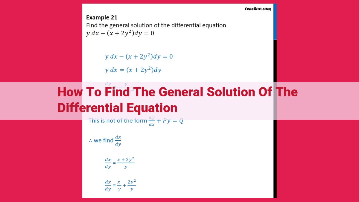
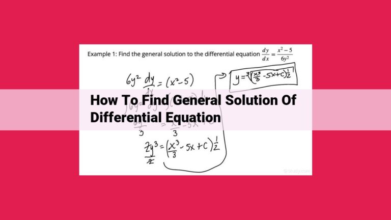
To find the general solution of a differential equation, classify its order, degree, linearity, and homogeneity. The general solution consists of the homogeneous solution found by solving the auxiliary equation, and the particular solution found by methods like undetermined coefficients or variation of parameters. Apply initial or boundary conditions to determine the particular solution. This step is crucial as it narrows down the general solution to a specific solution that satisfies the given conditions. By following these steps, you can effectively find the general solution of differential equations and explore their applications in various scientific and engineering disciplines.

Differential Equations: A Journey into the Dynamics of Change

In the realm of mathematics, differential equations hold a place of profound importance. They are equations that involve one or more functions and their derivatives, providing a powerful tool for describing and understanding the dynamic behavior of systems across a wide range of disciplines.

Differential equations have found indispensable applications in fields such as physics, engineering, biology, and economics. They allow scientists and researchers to model and analyze complex phenomena, such as the motion of celestial bodies, the flow of fluids, the growth of populations, and the behavior of financial markets.

From the humble beginnings of representing simple rates of change, differential equations have evolved into a sophisticated mathematical tool capable of unraveling the intricate dynamics of our world. Their ability to capture the essence of change has made them an indispensable ally in our quest for understanding the complexities of nature.

Classifying Differential Equations: A Journey Through the World of Equations

Welcome to the fascinating world of differential equations! As we delve into this concept, let’s first explore how we classify these equations to better understand their nature and behavior.

Order and Degree: The Foundation of Classification

The order of a differential equation refers to the highest order of derivative that appears in the equation. For instance, an equation with the highest derivative of the third order is called a third-order differential equation.

Similarly, the degree refers to the highest power of the highest derivative. A differential equation with the highest derivative raised to the power of two is considered a second-degree equation.

Linearity: A Tale of Two Equations

Differential equations can be classified as linear or nonlinear. Linear equations are characterized by their linearity in the dependent variable and its derivatives. In other words, the equation can be written as a sum of terms, each involving either the dependent variable or its derivatives multiplied by constant coefficients.

Nonlinear equations, on the other hand, deviate from this linearity. They involve non-linear terms, such as products of the dependent variable and its derivatives, or functions that are not linear.

Homogeneity: A Matter of Similarity

Another important classification is based on homogeneity. A differential equation is considered homogeneous if all its terms contain the dependent variable and its derivatives to the same degree. For example, the equation y” + xy’ + y = 0 is homogeneous because all terms involve y and its derivatives to the first power.

In contrast, nonhomogeneous equations contain terms that do not involve the dependent variable or its derivatives. These terms are often constants or functions of the independent variable. The equation y” + xy’ + y = x is nonhomogeneous due to the presence of the non-zero term x on the right-hand side.

Understanding these classifications is crucial for analyzing and solving differential equations. By categorizing them, we can apply appropriate methods and techniques to find their solutions. Stay tuned for future installments where we uncover the secrets of finding general and particular solutions to these equations!

General and Particular Solutions: The Key to Solving Differential Equations

In the world of differential equations, finding solutions is like solving a puzzle. And just like any puzzle, there are two main types of solutions: general and particular. Let’s dive into what they are and why they matter.

General Solution: A Blanket of Possibilities

Imagine you have a differential equation that represents a vast ocean of solutions. The general solution is like a gigantic net that captures all possible solutions for that equation. It’s a mathematical expression that contains an arbitrary function, representing the infinite variety of ways the solution can behave.

Why is the general solution so important? Because from this blanket of possibilities, we can pull out specific solutions that meet our specific needs.

Particular Solution: The Perfect Fit

A particular solution, on the other hand, is like a custom-tailored garment that perfectly fits a set of initial conditions or boundary conditions. These conditions are like constraints that narrow down the sea of possible solutions to a single, specific one.

Particular solutions are essential for modeling real-world phenomena, where we often have specific starting points or constraints. They allow us to make precise predictions and draw meaningful conclusions based on our differential equations.

In summary, general solutions provide the complete picture of all possible solutions, while particular solutions zoom in on the one that aligns perfectly with our specific problem. Together, they paint a vibrant tapestry of solutions, empowering us to tackle complex mathematical puzzles and gain insights into the world around us.

Finding the General Solution: A Guide to Solving Differential Equations

In the realm of mathematics, differential equations hold immense significance, providing a powerful tool for modeling and understanding complex phenomena in science, engineering, and beyond. Among their key features is the general solution, which represents a family of solutions that encompasses all possible scenarios.

To find the general solution, we embark on a journey that unfolds in several stages. First, we identify the type of equation, whether it’s linear or nonlinear, homogeneous or nonhomogeneous. This classification guides our choice of solution methods.

Next, we solve the homogeneous equation, which is the equation without a forcing term (often represented by the variables t or x). This step provides us with a foundational solution set.

Finally, we tackle the nonhomogeneous equation, which accounts for the forcing term. Here, our choice of method depends on the form of the nonhomogeneity:

• Method of Undetermined Coefficients: For constant coefficients, we assume a solution of the form that matches the nonhomogeneity, solving for its coefficients to obtain a particular solution.

• Variation of Parameters: For nonconstant coefficients, we introduce new functions into the assumed solution, leading us to a system of equations that can be solved to find the particular solution.

Unveiling the General Solution

Having obtained both the homogeneous and particular solutions, we combine them to arrive at the general solution. This solution represents the entire family of solutions that satisfy the differential equation. It allows us to explore the behavior of the system under various initial or boundary conditions.

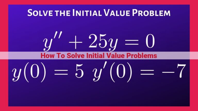
Initial Conditions: These conditions specify the values of the solution and its derivatives at a particular time or point. By substituting these values into the general solution, we can determine the unique solution that satisfies the given conditions.

Boundary Conditions: Similar to initial conditions, boundary conditions specify the values of the solution at specific points or intervals. They restrict the general solution to a specific family that satisfies the imposed constraints.

Understanding and confidently solving differential equations empowers us to delve deeper into the intricacies of our physical world. The ability to find the general solution is a cornerstone of this skill, unlocking the secrets held within these mathematical equations.

Solving Differential Equations: Mastering Initial and Boundary Conditions

Differential equations, the equations that describe how things change over time, play a pivotal role in fields like physics, engineering, and biology. They allow us to predict and analyze phenomena ranging from the trajectory of a rocket to the spread of an epidemic.

To fully understand differential equations, we need to explore the power of initial and boundary conditions. These conditions provide crucial information about the system’s behavior at specific points in time or space.

Initial Conditions:

• Concept: Initial conditions are values that describe the state of a system at a specific starting point.
• Significance: They allow us to find particular solutions that satisfy specific scenarios. For example, in a population growth model, the initial population size is an initial condition that affects the subsequent growth trajectory.

Boundary Conditions:

• Concept: Boundary conditions specify values that the solution must satisfy at specific points in space or time.
• Applications: They are essential in problems involving waves, heat transfer, and fluid dynamics. For instance, in a heat conduction problem, the temperature at the boundaries of a material may be fixed, imposing boundary conditions.

Using Initial and Boundary Conditions:

To solve differential equations, we must use initial and boundary conditions to obtain particular solutions that match real-world scenarios. These conditions serve as constraints that narrow down the possibilities, allowing us to find the unique solution that best describes the system.

Steps to Apply Initial and Boundary Conditions:

1. Find the general solution: This solution represents all possible solutions to the differential equation.
2. Substitute the initial or boundary conditions: Plug the given values into the general solution to obtain a particular solution.
3. Check your solution: Verify that the particular solution satisfies the differential equation and the given conditions.

Example:

Consider a simple differential equation that describes the growth of a population:

dP/dt = 0.5P

where P represents the population size.

If the initial population is 100, then the initial condition is P(0) = 100. To find the particular solution that satisfies this condition, we substitute P(0) = 100 into the general solution P = Ce^(0.5t). This gives us P = 100e^(0.5t), which represents the growth of the population over time.

By applying initial and boundary conditions, we unlock the power of differential equations to model and analyze real-world systems with precision. These constraints guide us toward specific solutions that accurately reflect the behavior of the system under study.