Mastering Differential Equation Solutions: A Comprehensive Guide

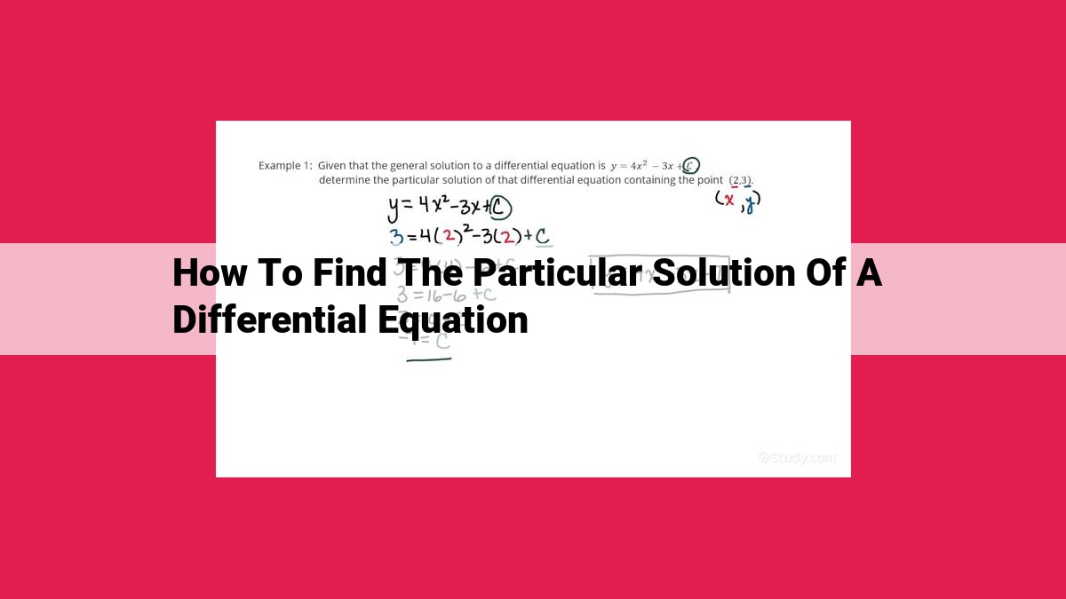
Finding a particular solution to a differential equation involves determining a function that satisfies both the equation and the given conditions. Several methods exist: Method of Undetermined Coefficients for equations with specific right-hand sides, Method of Variation of Parameters for non-constant coefficients, Green’s Function Method for non-homogeneous boundary conditions, Laplace Transform Method for solutions in different domains, and Fourier Series Method for periodic non-homogeneities.

Unveiling the Secrets of Differential Equations: A Guide to Finding Particular Solutions

Differential equations, the language of change, have countless applications in science, engineering, and everyday life. Finding their solutions, particularly particular solutions, is crucial for understanding real-world phenomena.

What are Particular Solutions in Differential Equations?

In differential equations, a general solution represents a family of solutions, encompassing an infinite number of possibilities. Each specific solution from this family that satisfies given initial or boundary conditions is known as a particular solution. These solutions provide valuable insights into the specific behavior of a system under particular conditions.

Methods for Finding Particular Solutions

Various methods exist to find particular solutions, each tailored to specific types of differential equations and non-homogeneous terms. Here are some commonly used techniques:

• Method of Undetermined Coefficients: This method involves guessing a particular solution based on the form of the non-homogeneous term. It’s often effective when dealing with constant coefficients or simple exponential and trigonometric terms.

• Method of Variation of Parameters: When the method of undetermined coefficients fails, variation of parameters constructs a particular solution as a linear combination of homogeneous solutions. This technique utilizes the Wronskian, a determinant that measures the linear independence of solutions.

• Green’s Function Method: The Green’s function is a special function that characterizes the response of a system to a specific input. Using convolution, this method relates the non-homogeneous term to the particular solution.

• Laplace Transform Method: This method involves transforming the differential equation into an algebraic equation in the frequency domain using the Laplace transform. The particular solution is then obtained by applying the inverse Laplace transform.

• Fourier Series Method: When the non-homogeneous term is periodic, the Fourier series method expresses it as a sum of sinusoidal terms. By using Parseval’s theorem, a particular solution is constructed as a sum of sinusoidal terms with appropriate coefficients.

Unveiling the Method of Undetermined Coefficients: A Journey to Find Particular Solutions

In the realm of differential equations, finding particular solutions is crucial for unlocking the secrets of complex systems. Among the methods available, the Method of Undetermined Coefficients stands out as a powerful tool in the hands of skilled mathematicians.

This method shines when the non-homogeneous term (the part that doesn’t contain the unknown function) takes on a predictable form, such as polynomials, exponentials, or trigonometric functions. The key principle underlying this method is the ****educated guess_: we assume a particular solution that has the same form as the non-homogeneous term, but with unknown coefficients.

Steps to Guess a Particular Solution:

1. Identify the form of the non-homogeneous term (e.g., polynomial, exponential).
2. Write down a general expression for a particular solution that matches this form, but with unknown coefficients.
3. Substitute this expression into the differential equation and solve for the coefficients.
4. Multiply the particular solution by an integrating factor (if necessary) to simplify the equation.

The integrating factor is a function that, when multiplied by a differential equation, transforms it into an equation that is easier to solve. In the Method of Undetermined Coefficients, the integrating factor is often a power of e or the _Wronskian, which measures the independence of solutions to homogeneous equations.

By meticulously applying these steps, mathematicians can find particular solutions that satisfy differential equations and unlock the secrets of complex systems, from modeling mechanical vibrations to predicting the behavior of electric circuits.

Method of Variation of Parameters

• Explain why the method of undetermined coefficients may fail.
• Describe the concept of constructing a particular solution as a linear combination of homogeneous solutions.
• Highlight the role of the Wronskian and integrating factor.

The Method of Variation of Parameters: Finding a Particular Solution When the Undetermined Coefficients Fall Short

If you’ve been working with differential equations, you’ve likely encountered the Method of Undetermined Coefficients, which can be a handy tool for finding particular solutions. However, there are times when this method falls short. That’s where the Method of Variation of Parameters comes in as a game-changer.

Imagine you’re dealing with a non-homogeneous differential equation like this:

y'' + p(x)y' + q(x)y = g(x)

where g(x) is a nasty non-zero function that’s throwing a wrench into your efforts to find a particular solution. The Undetermined Coefficients Method would chuckle at this challenge, but the Method of Variation of Parameters is here to save the day.

The Core Idea: Constructing a Solution from Homogeneous Solutions

The key insight behind this method is that we can construct a particular solution as a linear combination of the homogeneous solutions, which are the solutions to the corresponding homogeneous equation (i.e., when g(x) = 0). Let’s call these homogeneous solutions y_1(x) and y_2(x).

Our particular solution will look something like this:

y_p(x) = u(x)y_1(x) + v(x)y_2(x)

where u(x) and v(x) are functions to be determined.

Determining the Functions with Wronskian and Integrating Factor

Here’s the magic: The Wronskian, a determinant that captures the relationship between the homogeneous solutions, plays a crucial role. If the Wronskian is not zero, it ensures that the homogeneous solutions are linearly independent, which is essential for this method.

Now, we need to find u(x) and v(x) by solving a system of equations, which involves an integrating factor. This factor ensures that the equations become exact differential equations, making them much easier to solve.

A Note on Applicability

The Method of Variation of Parameters shines when the Undetermined Coefficients Method fails, typically when the non-homogeneous term g(x) is not of a special form (e.g., polynomials, exponentials, or their combinations). It’s a versatile technique that complements the Undetermined Coefficients Method, giving you a powerful arsenal for tackling a wide range of differential equations.

The Green’s Function Method: A Powerful Tool for Solving Differential Equations

In the realm of differential equations, finding particular solutions holds profound significance. It enables us to craft solutions tailored to specific input functions, providing valuable insights into how systems behave under various conditions. Among the various methods available, the Green’s Function Method stands out for its effectiveness and versatility.

The Green’s function, denoted by G(x, t), embodies the response of a system to an impulse input. It encapsulates the system’s inherent properties and its behavior in response to external stimuli. By utilizing the Green’s function, we can establish a direct link between the input and output of the system.

To harness the power of the Green’s function, we employ a technique known as convolution. Convolution involves integrating the product of the input function and the Green’s function over the entire time domain. The result of this operation yields the particular solution.

Mathematically, it can be expressed as:

y(t) = ∫[G(x, t) * f(x)]dx

where:

• y(t) is the particular solution
• G(x, t) is the Green’s function
• f(x) is the input function

The Green’s function method offers a powerful approach to solving differential equations in various fields, including physics, engineering, and mathematics. By establishing the relationship between input and output, it enables us to predict system behavior and design solutions that meet specific requirements.

Laplace Transform Method

• Explain the transformation between the time domain and frequency domain.
• Describe how the Laplace transform can convert a differential equation into an algebraic equation.
• Discuss the use of the inverse Laplace transform to obtain the particular solution.

Laplace Transform Method: Unlocking the Power of Transformation in Differential Equations

In the realm of differential equations, the Laplace transform emerges as a transformative tool that transcends the boundaries of time and frequency domains. This powerful technique unravels the intricacies of complex equations, offering a pathway to finding particular solutions with unmatched elegance.

The Laplace transform, a mathematical operator, whisks functions from the time domain, where they reside as intricate phenomena, into the frequency domain, where they reveal their hidden patterns as algebraic equations. This transformation harnesses the essence of time and frequency, allowing us to view differential equations from a fresh perspective.

Armed with the Laplace transform, we can effortlessly convert a differential equation into a much more manageable algebraic counterpart. This transformation opens up a treasure trove of tools from algebra, enabling us to solve the equation with ease. Once we have tamed the equation in the frequency domain, the inverse Laplace transform, the time-bending counterpart, gracefully transports us back to the time domain, where we retrieve the elusive particular solution.

The Laplace transform method shines particularly bright in the presence of functions that are initially nasty and seemingly inscrutable. Discontinuous functions, step functions, and periodic functions, which once held us captive, now tremble before the might of the Laplace transform. Their hidden patterns, once shrouded in mystery, are laid bare, revealing their true nature and yielding to our relentless pursuit of solutions.

Embark on the Laplace Transform Adventure:

1. Step into the Time-Frequency Nexus: Begin by applying the Laplace transform to your differential equation, watching in awe as time morphs into frequency, and complexity yields to simplicity.

2. Conquer the Algebraic Enigma: Flex your algebraic muscles as you tackle the transformed equation, wielding your newfound power to solve for the unknown coefficients.

3. Return to the Temporal Realm: Perform the inverse Laplace transform, a magical incantation that summons your particular solution back from the frequency domain, granting you the wisdom to unravel the secrets of your equation.

The Laplace transform method, a beacon of hope in the labyrinth of differential equations, empowers us to conquer even the most intimidating mathematical challenges. Embrace its transformative power, and witness the boundaries of your understanding expand as you master the art of finding particular solutions with unparalleled precision.

Finding Particular Solutions in Differential Equations: Methods to Unravel the Equations’ Secrets

In the realm of differential equations, finding particular solutions is like solving a thrilling mystery. Just as detectives use various methods to unravel a crime, mathematicians employ different techniques to uncover the secrets hidden within these equations.

Fourier Series Method: Unlocking Patterns in Periodic Systems

When dealing with non-homogeneous differential equations that have periodic terms, the Fourier Series Method emerges as a powerful tool. This method harnesses the principles of Fourier series, a mathematical technique that decomposes periodic functions into an elegant symphony of orthogonal functions known as sinusoids.

The Magic of Fourier Series

The Fourier series method begins by representing the non-homogeneous term of the differential equation as a sum of sinusoids. These sinusoidal terms oscillate at different frequencies, capturing the inherent periodicity of the non-homogeneous term. By doing so, we essentially break down the complex non-homogeneous term into a series of simpler sinusoidal pieces.

Constructing the Particular Solution

With the non-homogeneous term decomposed, we can now construct a particular solution to the differential equation. This particular solution is also represented as a sum of sinusoidal terms, each term corresponding to a frequency present in the non-homogeneous term. The coefficients of these sinusoidal terms are determined using Parseval’s theorem, which provides a way to calculate the energy of a signal represented by a Fourier series.

A Harmonious Symphony

The Fourier series method allows us to find particular solutions to differential equations with periodic non-homogeneous terms. It transforms complex periodic functions into a symphony of sinusoids, unlocking the secrets of these equations through a delicate balance of mathematical techniques.