Maximize Problem-Solving Efficiency With Linearization Techniques

Linearization transforms complex equations into simpler linear equations for easier solutions. It involves approximating nonlinear functions with tangent lines or Taylor series, expanding them as power series with the first few terms representing the linear approximation. Linear approximation simplifies calculations, allowing for efficient estimation of function values near specific points. By utilizing linearization techniques like Taylor series or first- and second-order linearization, it becomes possible to solve complex problems by reducing them to solvable linear equations.

Linearization: The Art of Simplifying Non-Linear Equations

In the realm of mathematics, linear equations reign supreme. They are simple, straightforward, and immensely useful in solving a myriad of problems. However, what happens when we encounter equations that refuse to conform to this linear simplicity? Enter the concept of linearization, a powerful technique that transforms complex equations into manageable linear approximations.

Linearization: A Bridge to Linearity

Linearization is the process of approximating a non-linear function with a linear equation. It’s like taking a curvy road and straightening it out, making it easier to navigate and analyze. This approximation is crucial because it allows us to apply the familiar tools of linear algebra to solve problems involving non-linear equations.

Why Linearise?

Solving non-linear equations can be a tedious and time-consuming task. By linearizing them, we can simplify the process significantly. Moreover, linearization can provide valuable insights into the behavior of non-linear functions, making them more predictable and manageable.

Linear Approximation: A Powerful Tool for Approximating Non-Linear Functions

In the realm of mathematics, linear equations play a pivotal role. Their simplicity and ease of solution make them an indispensable tool for solving a wide range of problems. However, the world around us is often governed by non-linear functions, which pose a greater challenge to our mathematical prowess. Enter linear approximation, a technique that empowers us to approximate these complex functions with good ol’ linear equations.

Concept 1: Linear Approximation

What is linear approximation, you ask? It’s a clever way of approximating a non-linear function with a linear one. Just imagine your non-linear function as a curvy road. Linear approximation is like building a straight line that closely follows the road around a specific point. This straight line, known as the tangent line, provides a local approximation of the non-linear function.

How does it work? The beauty of linear approximation lies in its simplicity. We determine the slope of the non-linear function at the desired point and use it to define the equation of the tangent line. This tangent line becomes our linear approximation, providing an estimate of the original function’s value near that point.

Example:

Let’s say you have a function f(x) = x^2. If you want to approximate the value of f(x) near x = 2, simply calculate the slope of the function at x = 2, which is 4. The tangent line equation becomes y = 4(x – 2) + 8. This linear approximation will provide a reasonably accurate estimate of f(x) for values of x close to 2.

Related Concept: Tangent Line Approximation

• Explain the tangent line approximation and how it relates to linear approximation.
• Show how the tangent line approximation can be used to approximate the value of a function at a given point.

Tangent Line Approximation: Your Fast Track to Approximating Non-Linear Functions

In the realm of mathematics, we often encounter non-linear equations that can be quite challenging to solve exactly. But fear not, dear reader! Linearization techniques come to our rescue, providing us with a powerful tool to approximate these complex functions with much simpler linear ones.

One such technique is the tangent line approximation. This approach involves drawing a tangent line to a non-linear function at a specific point. The tangent line is a straight line that approximates the function’s behavior near that point.

How does it work?

Imagine a function that curves through the coordinate plane. At any given point on the curve, we can construct a tangent line that touches the curve at that point. This tangent line is defined by an equation of the form:

y = f(a) + f'(a)(x - a)

where a is the point of tangency, f(a) is the function value at a, and f'(a) is the derivative of the function at a.

Why is it useful?

The tangent line approximation is incredibly valuable because it allows us to approximate the value of the non-linear function at any point x near a. We simply plug x into the tangent line equation and solve for y:

y ≈ f(a) + f'(a)(x - a)

This approximation is particularly accurate when x is close to a, as demonstrated by the following example:

Suppose we want to approximate the value of the function f(x) = e^x at x = 1.1.

• Evaluate the function and its derivative at a = 1: f(1) = e^1 = 2.71828 and f'(1) = e^1 = 2.71828
• Substitute into the tangent line equation: y = 2.71828 + 2.71828(x – 1)
• Approximate f(1.1): y ≈ 2.71828 + 2.71828(0.1) = 3.0

Concept 2: The Power of the Taylor Series

So far, we’ve explored linear approximation, a powerful tool for simplifying complex functions. But let’s dive even deeper into the world of approximations with the Taylor series. Picture this: the Taylor series is like a magical formula that can transform any well-behaved function into a series of simpler terms.

At the heart of the Taylor series lies the idea of a power series, a special kind of polynomial that goes on forever. The Taylor series takes a function and expands it into this power series around a specific point. The first few terms of the Taylor series give us a very accurate approximation of the function near that point.

One of the coolest things about the Taylor series is that it can turn any non-linear function into a linear one. How’s that possible? Well, if we only consider the first two terms of the Taylor series, we end up with a linear approximation of the function. It’s like finding the best straight line that fits the curve of the function at a particular point.

Think of it this way: the Taylor series is like a Swiss Army knife for function approximation. It can handle even the most complex functions and provide us with a simplified approximation that can make our calculations much easier. So, when you encounter a non-linear equation that gives you a headache, don’t despair – reach for the Taylor series and let it work its magic!

First-Order Linearization: Simplifying the Complex

In the realm of mathematics, linear equations are a cornerstone of understanding complex phenomena. They allow us to represent relationships between variables in a straightforward way. However, many real-world scenarios involve non-linear functions that are more intricate and challenging to solve.

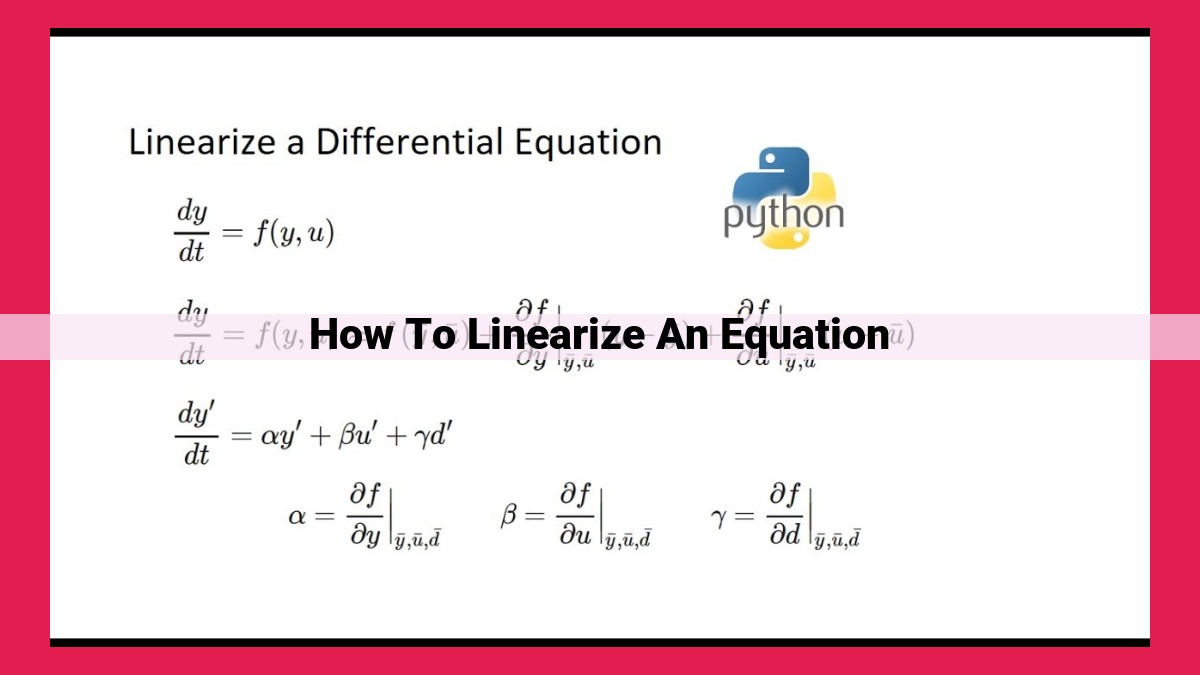
Enter linearization, a technique that provides a clever way to approximate these non-linear equations with linear ones, making them more manageable. Among its various forms is the first-order linearization, a simplified approach that leverages the power of the Taylor series.

The Taylor series is an intriguing mathematical concept that represents a function as an infinite power series. With its first two terms, we obtain a formula that enables us to linearize a non-linear function around a specific point.

Visualizing the Linearization Process

To grasp the essence of first-order linearization, imagine a non-linear function as a curvy path. At a particular point on this path, you can draw a straight line, known as a tangent line, which closely approximates the function’s behavior near that point. This tangent line is the first-order linearization of the non-linear function.

Approximating Function Values with First-Order Linearization

The beauty of first-order linearization lies in its ability to estimate function values close to the chosen point. By plugging the point’s value into the equation of the tangent line, you obtain an approximation of the function’s value at that point.

A Real-World Illustration

Let’s say you have a function representing the trajectory of a projectile thrown into the air. The non-linear equation describes the projectile’s height over time. Using first-order linearization, you can approximate the projectile’s height at any given time within a reasonable range around the initial launch point.

Benefits and Applications

First-order linearization is a valuable tool for scientists, engineers, and economists who work with complex non-linear equations. It provides a quick and efficient way to approximate function values, enabling them to gain insights and make predictions without the need for intensive numerical methods.

In conclusion, first-order linearization is an accessible and powerful technique that unlocks the understanding of non-linear systems. By harnessing the simplicity of linear approximations, it empowers us to navigate complex mathematical landscapes and uncover valuable information from otherwise intricate functions. Its applications span across diverse fields, from modeling physical phenomena to analyzing economic trends.

Unveiling the Power of Linearization: Approximating Non-linear Equations with Ease

In the realm of mathematics, linear equations hold a fundamental place. They represent the simplest and most well-behaved functions, making them easy to solve. However, in the real world, we often encounter non-linear equations that defy simple solutions. This is where linearization steps in, offering a valuable tool to approximate these complex functions.

Linear Approximation: A First Glance

Consider a non-linear function, such as the square root function. It’s not as straightforward to solve as a linear equation. However, we can linearize it by approximating it with a straight line that closely follows its curve near a specific point. This straight line is called the tangent line, and it provides a convenient way to approximate the value of the original function at that point.

Exploring the Taylor Series

The Taylor series takes linearization to the next level. It allows us to represent a function as a sum of infinitely many terms, each involving a derivative of the function at a given point. The first two terms of this series constitute the first-order linearization, which we’ve discussed earlier.

The Second-Order Linearization: A More Refined Approximation

Moving beyond the first-order linearization, we have the second-order linearization. This involves using the first three terms of the Taylor series, resulting in a more accurate approximation. It captures not only the slope of the tangent line but also its curvature. This enhanced precision makes the second-order linearization a powerful tool for approximating functions with greater complexity.

Benefits of Linearization: A Problem-Solver’s Ally

Linearization provides several key benefits:

• Simplified Equations: It transforms non-linear equations into manageable linear equations, making them easier to solve.
• Accurate Approximations: Linearization offers reliable approximations, especially when the non-linear function is close to linear near the point of approximation.
• Versatile Applications: Linearization finds applications in diverse fields, including economics, engineering, and physics, where it helps approximate complex phenomena.

Linearization is an indispensable tool for dealing with non-linear equations. It provides a systematic way to approximate complex functions with simpler linear equations, offering valuable insights into their behavior. Whether it’s through first-order or second-order linearization, this technique empowers us to unlock the mysteries of non-linearity, making problem-solving more accessible and efficient.