The Ultimate Guide To Optimizing Labor Productivity: Marginal Product Of Labor (Mpl) Explained

Marginal Product of Labor (MPL) measures the change in output resulting from an additional unit of labor input, holding other inputs constant. The formula is Δoutput / Δlabor. Accurate MPL measurement requires a smooth and continuous production function. MPL is represented by the slope of the short-run production function and is subject to diminishing returns as labor increases. Long-run MPL may differ from short-run MPL due to specialization and resource availability. MPL applies to variable inputs, while fixed inputs remain constant. MPL is related to Marginal Revenue Product (MRP), which represents the market value of labor’s contribution. Understanding MPL is crucial for maximizing labor productivity and firm optimization.

The Enigma of Marginal Product of Labor: Unveiling the Essence of Labor Productivity

In the realm of economics, the understanding of labor productivity is crucial for businesses striving to optimize their operations. At the heart of this concept lies an enigmatic metric known as the marginal product of labor (MPL).

Introducing the Marginal Product of Labor

MPL, simply put, measures the additional output produced by an additional unit of labor while holding all other factors of production constant. It’s a vital indicator of how efficiently labor is being utilized within an organization. By understanding MPL, businesses can make informed decisions about staffing levels, resource allocation, and production strategies to maximize their efficiency and profitability.

The Formula Unveiled

Calculating MPL is a straightforward process. It’s determined by dividing the change in output (ΔQ) by the change in labor (ΔL):

MPL = ΔQ / ΔL

This formula allows businesses to quantify the exact contribution of each additional worker to the overall production process.

Unveiling the Significance of Conditions

For accurate MPL measurement, certain conditions must be met:

• Smoothness of the Production Function: The relationship between labor input and output should be continuous and devoid of any sudden jumps or irregularities.
• Continuity of the Production Function: The MPL should change gradually as labor increases, without any abrupt shifts or discontinuities.

Meeting these conditions ensures that MPL accurately reflects the marginal contribution of labor to production.

Interwoven with the Short-Run Production Function

In the short run, MPL is directly related to the slope of the production function. As labor increases, the slope will typically rise, indicating that each additional worker contributes more output than the previous one. However, this relationship has its limits.

Diminishing Returns and Its Impact

As labor continues to increase, the Law of Diminishing Returns kicks in. This means that the MPL will eventually start to decline, indicating that each additional worker contributes less output than the previous one. This phenomenon is caused by the diminishing returns from adding more labor while keeping other factors constant.

Long-Run Dynamics: A Different Perspective

In the long run, MPL behaves differently due to factors like specialization, division of labor, and resource availability. In this scenario, MPL can increase over time as workers become more skilled and specialized, and better production methods are implemented.

Variable vs. Fixed Inputs: The Distinction

MPL measures the change in output due to changes in variable inputs (e.g., labor) while holding fixed inputs (e.g., capital) constant. This distinction is essential for accurately understanding the true relationship between labor and output.

The Interplay with Marginal Revenue Product

Finally, MPL and marginal revenue product (MRP) are closely related concepts. MRP represents the market value of labor’s contribution and can differ from MPL due to market forces. Understanding the relationship between MPL and MRP is crucial for firms seeking to optimize their labor utilization.

Calculating Marginal Product of Labor: Unveiling the Value of Human Contribution

In the realm of economics, understanding the marginal product of labor (MPL) is crucial for deciphering the productivity and efficiency of labor within a firm. MPL quantifies the additional output yielded by employing one extra unit of labor while keeping other factors of production constant.

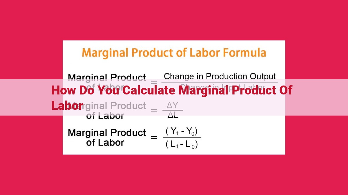
Formula for Calculating MPL: A Simple Yet Powerful Equation

The mathematical formula for MPL is elegantly straightforward:

MPL = ΔOutput / ΔLabor

Where:

• ΔOutput represents the change in output (produced goods or services)
• ΔLabor represents the change in the quantity of labor employed

For instance, if a firm produces 100 units of output with 10 workers and 110 units of output with 11 workers, the MPL for the 11th worker is 10 units.

Conditions for Accurate MPL Measurement

It’s essential to note that two crucial conditions must be met for accurate MPL measurement:

1. Smoothness of the Production Function: The production function, which depicts the relationship between output and labor, should be smooth and continuous. This ensures that small changes in labor quantity result in predictable changes in output.

2. Continuity of the Production Function: The production function should be continuous, meaning that it has no abrupt jumps or discontinuities. This ensures thatMPL can be calculated at any given level of labor input.

By adhering to these conditions, we can confidently derive accurate MPL values.

Conditions for Accurate MPL Measurement

To obtain an accurate measurement of the Marginal Product of Labor (MPL), certain conditions must be met regarding the production function. A production function describes the relationship between the quantity of inputs (like labor) and the resulting output. For MPL measurement to be reliable, the production function should exhibit the following characteristics:

• Smoothness: The production function should be a smooth, continuous curve without any abrupt changes or discontinuities. This implies that output changes gradually as labor input increases. If the function is not smooth, it may be difficult to determine the exact slope, which represents the MPL.

• Continuity: The production function should be continuous, meaning there are no sudden jumps or gaps in the curve. This ensures that the MPL remains well-defined for all possible labor inputs. A discontinuous function would make it challenging to calculate the slope accurately.

Relationship between Marginal Product of Labor and the Short-Run Production Function

In the realm of microeconomics, the marginal product of labor (MPL) plays a pivotal role in understanding how firms maximize their output. It represents the additional output generated by employing one more unit of labor, ceteris paribus.

A firm’s short-run production function outlines the relationship between the amount of labor employed and the corresponding output level. Interestingly, the MPL is directly represented by the slope of this production function. Let’s delve deeper into this connection.

Imagine a production function that plots output on the y-axis and labor on the x-axis. The slope of this function at any given point indicates the MPL at that particular level of labor. This is because the slope measures the change in output (y-axis) relative to the change in labor (x-axis), which is precisely the definition of MPL.

In other words, the slope of the production function represents the incremental output generated by hiring one more unit of labor. This information is invaluable for firms seeking to optimize their labor force and maximize their production efficiency. By understanding the MPL, firms can make informed decisions about hiring levels and resource allocation to achieve their desired output targets.

The Law of Diminishing Returns and Its Impact on Marginal Product of Labor (MPL)

In the realm of economics, the marginal product of labor (MPL) measures the incremental output generated by adding one additional unit of labor while holding all other inputs constant. However, this relationship is not always linear; the Law of Diminishing Returns asserts that as more labor is added to a production process, the marginal product of each additional unit tends to decrease.

Imagine a farmer tending to a field. Initially, adding more workers leads to a significant increase in output as they can efficiently cultivate more land. However, as the number of workers continues to grow, the available land becomes more crowded, and each additional worker contributes less to the overall harvest. This is because the fixed inputs, such as land and capital, become limiting factors.

The Law of Diminishing Returns has profound implications for businesses and policymakers. As labor costs rise, firms must carefully consider the MPL of each additional worker to ensure that they are still generating a profitable return on their investment. Governments, on the other hand, must be mindful of the potential impact of increasing the labor supply on overall economic growth.

In conclusion, understanding the Law of Diminishing Returns is crucial for optimizing labor productivity and making informed decisions in the labor market. It highlights the importance of balancing the addition of labor with other inputs to maximize output and efficiency.

Long-Run vs. Short-Run MPL: A Tale of Specialization and Resource Availability

In the realm of economics, understanding the Marginal Product of Labor (MPL) is crucial for unraveling the intricate tapestry of labor productivity and firm optimization. Previously, we delved into the definition, formula, and significance of MPL. Now, let us embark on a captivating journey to explore the intriguing differences between Long-Run and Short-Run MPL.

Picture a scenario where you hire an additional worker in your factory. Initially, you may witness a surge in output as the new worker joins forces with the existing team. This immediate increase in output is attributed to short-run MPL. However, as you continue to add more workers while keeping other factors constant, a curious phenomenon unfolds. The incremental output generated by each additional worker gradually diminishes. This is where the Law of Diminishing Returns comes into play, indicating a finite limit to the productivity gains from adding more labor.

Now, consider a scenario where you have the luxury of long-run planning. In the long run, you can adjust not only labor but also other resources like capital and technology. This flexibility creates a different landscape for MPL. Specialization, division of labor, and access to new resources can unlock significant productivity gains. As workers specialize in specific tasks and collaborate effectively, their collective output can skyrocket. Additionally, investments in capital and technological advancements can further amplify productivity, leading to a higher long-run MPL.

The key distinction between long-run and short-run MPL lies in the availability of time and resources. In the short run, firms are constrained by existing resources, while in the long run, they have the freedom to adapt and optimize their production processes. This flexibility allows firms to overcome diminishing returns and achieve sustainable productivity growth.

Understanding the nuances of Long-Run and Short-Run MPL empowers businesses with valuable insights for strategic workforce planning and resource allocation. By tailoring their hiring and investment decisions accordingly, firms can maximize labor productivity, optimize costs, and achieve their long-term goals.

Variable vs. Fixed Inputs

Understanding the concept of marginal product of labor (MPL) requires a clear distinction between variable and fixed inputs. Variable inputs are factors of production whose quantity can be easily adjusted in the short run. Labor is a classic example of a variable input since firms can hire or lay off workers as needed.

In contrast, fixed inputs are factors of production whose quantity cannot be easily changed in the short run. Capital is a common fixed input because it takes time and significant investment to acquire and install machinery, buildings, and other capital assets.

MPL measures the change in output resulting from a change in variable inputs, holding fixed inputs constant. This means that MPL captures the additional output produced as a firm adds more labor while keeping capital and other fixed inputs unchanged. This distinction is crucial for understanding how firms optimize their production processes.

Relationship with Marginal Revenue Product (MRP)

Understanding the Market Value of Labor

• Marginal Revenue Product (MRP) measures the additional revenue generated by hiring one more unit of labor.
• It represents the true market value of labor’s contribution to the firm.

****Distinguishing MRP from MPL

• While Marginal Product of Labor (MPL) measures the physical output produced by an additional unit of labor, MRP considers the monetary value of that output.
• Market forces, such as product prices and demand, influence MRP.
• MRP and MPL may differ if the firm cannot sell all its output at the assumed market price.

Implications for Firm Optimization

• Profit-maximizing firms hire labor up to the point where MRP equals the wage rate.
• This ensures that the firm is using labor efficiently and generating the maximum possible revenue.
• Understanding the relationship between MRP and MPL helps firms make informed decisions about labor allocation and production levels.