Mastering Function Graphing: Key Features, Calculus, Transformations, And Sketching Accuracy

In sketching a function’s graph, first determine its key features: intercepts, symmetry, maximums/minimums, and asymptotes. Analyze its behavior using calculus (derivatives and second derivatives) to find intervals of increase/decrease and concavity. Understand transformations (shifts, dilations, reflections, rotations) and their effects on the graph. Combine these analyses to create a comprehensive sketch, paying attention to details and accuracy.

Briefly define mathematical functions and their components (input, output, domain, and range).

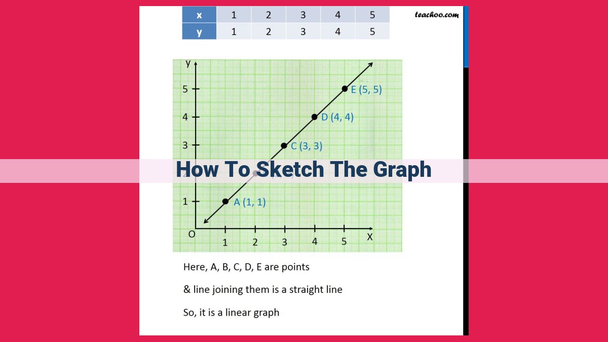
How to Sketch the Graph of a Mathematical Function: A Beginner’s Guide

Embark on this captivating journey to master the art of sketching mathematical functions. These functions are like magical blueprints that describe the relationship between two variables, revealing their inputs and outputs. They are governed by domains and ranges, boundaries that define their playground.

Identifying Key Features

Unravel the secrets of key features that shape the graph’s silhouette. First, pinpoint the intercepts, where the graph gracefully touches the axes. Symmetry plays a crucial role, too. Discover functions that mirror themselves across the origin, x-axis, or y-axis.

Analyzing Function Behavior

Peer into the function’s behavior to discern patterns and trends. Locate maximum and minimum points, the peaks and valleys of the graph. Asymptotes, elusive lines, tantalizingly approach but never meet, marking the graph’s boundaries.

Using Calculus to Sketch the Graph

For those eager to delve deeper, calculus provides a powerful tool. The derivative reveals intervals of increasing and decreasing, while the second derivative unveils the graph’s curvature.

Transformations of Functions

Witness the extraordinary power of transformations. Translations gracefully shift the graph across the coordinate plane. Dilations stretch or shrink it, altering its scale. Reflections mirror the graph, inverting its orientation.

Putting It All Together

Now, let’s orchestrate the symphony of key features, function behavior, and transformations. By harmonizing these elements, you’ll paint a meticulously accurate portrait of the function.

Mastering the art of sketching mathematical functions is a rewarding endeavor. Practice diligently and soon you’ll effortlessly unveil the hidden wonders within these equations. Remember, patience and curiosity are your guiding lights on this illuminating path.

Intercepts: Explain how to find the x- and y-intercepts where the graph crosses the axes.

Intercepts: Pinpointing Where the Graph Meets the Axes

In the world of mathematical functions, intercepts play a pivotal role in understanding the function’s behavior. Intercepts are the points where the graph of a function crosses either the x-axis or the y-axis.

To find the x-intercepts, set the y-coordinate to zero (y = 0) in the function equation. The resulting values of x will give you the x-intercepts where the graph crosses the x-axis. For instance, if you have the function f(x) = x² – 4, setting y = 0 and solving for x gives x = ±2, which means the graph crosses the x-axis at (-2, 0) and (2, 0).

Similarly, to find the y-intercepts, set the x-coordinate to zero (x = 0) in the function equation. The resulting value of y will give you the y-intercepts where the graph crosses the y-axis. Using the same function f(x) = x² – 4, setting x = 0 gives y = -4, indicating that the graph crosses the y-axis at (0, -4).

Intercepts are crucial because they provide valuable information about the function. They can help you determine the function’s domain (the set of all possible x-values), range (the set of all possible y-values), and symmetry. Additionally, intercepts allow you to identify the starting points of the graph, making it easier to sketch a more accurate representation.

Symmetry: Unlocking the Patterns of Mathematical Functions

Identifying the Three Types of Symmetry

In the realm of mathematics, functions often exhibit intriguing symmetry properties that provide valuable insights into their behavior. Symmetry refers to the existence of a reflection or rotation that leaves the function unchanged. There are three main types of symmetry to consider:

• Origin Symmetry: When a function is symmetric with respect to the origin, it appears as if it has been flipped across both the x-axis and y-axis. This mirrored image around the point (0, 0) indicates that if you replace x with -x and y with -y, the function remains the same. For example, the function f(x) = x² exhibits origin symmetry because f(-x) = (-x)² = x².

• X-Axis Symmetry: A function with x-axis symmetry has a mirror image about the x-axis. This means that if you reflect the graph across the x-axis, it will look exactly the same. To test for x-axis symmetry, replace y with -y in the function. If the result is still the same, the function is symmetric with respect to the x-axis. A classic example is the function f(x) = |x|, which represents the absolute value of x.

• Y-Axis Symmetry: In contrast to x-axis symmetry, y-axis symmetry occurs when a function is mirrored along the y-axis. This means that replacing x with -x leaves the function unchanged. For instance, the function f(x) = sin(x) has y-axis symmetry because f(-x) = sin(-x) = -sin(x), which is the same as f(x) but with a flipped sign.

Identifying Maximum and Minimum Points

In the realm of mathematical functions, maximums and minimums are the peaks and valleys of a graph, where the function reaches relative high and low points, respectively. Imagine a roller coaster ride, with its exhilarating highs and disheartening lows. Similarly, functions have these crucial turning points that reveal their behavior.

To find maximums and minimums, we delve into calculus, a powerful tool that allows us to analyze the function’s slope. The derivative, a mathematical cousin of the slope, tells us the rate of change of the function at any given point. When the derivative is zero, the function is either at a maximum or a minimum.

To determine which it is, we compare the derivative values on either side of the zero point. If the derivative changes from negative to positive around the zero, we have a local minimum. If it changes from positive to negative, it’s a local maximum. These turning points are like signposts on a mathematical journey, guiding us to the most prominent features of a graph.

Asymptotes: Guiding Lights to Function Boundaries

As we delve into the intricacies of mathematical functions, we encounter enigmatic lines that seem to draw near but never quite touch the graph. These ethereal lines are known as asymptotes, and they serve as valuable guides to the function’s behavior at infinity.

Vertical Asymptotes: Barriers of Discontinuity

Vertical asymptotes are towering lines parallel to the y-axis that represent points where the function is undefined. These discontinuities arise when the denominator of a rational function becomes zero. For instance, the function f(x) = 1/(x-2) has a vertical asymptote at x = 2 because dividing by zero is mathematically inadmissible.

Horizontal Asymptotes: Limits of Distant Horizons

In contrast to vertical asymptotes, horizontal asymptotes are lines parallel to the x-axis that indicate the function’s behavior as x approaches infinity or negative infinity. These asymptotes represent the horizontal limits of the function. For example, the function f(x) = (x^2 + 1)/(x^2 + 2) has a horizontal asymptote at y = 1 because as x grows infinitely large or small, the fraction approaches 1.

Slant Asymptotes: Bridging Gaps

Slant asymptotes, also known as oblique asymptotes, are diagonal lines that occur when the degree of the numerator is greater than or equal to the degree of the denominator of a rational function, with a remainder that is a first-degree polynomial. These asymptotes represent the graph’s limiting behavior as x approaches infinity or negative infinity. For instance, the function f(x) = (x^2 + 2x + 1)/(x + 1) has a slant asymptote at y = x + 1, which can be found by dividing the polynomial entirely.

Identifying asymptotes is crucial for sketching accurate graphs of functions. They provide visual cues to the function’s domain, range, and limits, enabling us to better understand its behavior across the entire number line.

Derivative Analysis: Unveiling the Secrets of Function Behavior

In the realm of calculus, the derivative plays a pivotal role in deciphering the hidden secrets of mathematical functions. Just as an artist uses brushstrokes to paint a masterpiece, the derivative reveals the contours of a function’s graph, allowing us to grasp its intricate nature.

The derivative measures the rate of change of a function. By analyzing its sign, we can identify intervals of increasing or decreasing. A positive derivative indicates an upward trend, while a negative derivative signals a downward trajectory. These insights paint a clear picture of the function’s overall shape.

Furthermore, the derivative provides a gateway to understanding concavity. Concavity refers to the curvature of the graph. A positive second derivative indicates that the graph curves upward (convex), while a negative second derivative indicates that it curves downward (concave). These subtleties add depth and dimension to the graph, shaping its overall appearance.

By combining the insights gained from derivative analysis with the techniques for identifying key features and transformations, we embark on a journey of discovery. We unravel the mysteries of mathematical functions, revealing their hidden patterns and behaviors. Armed with this knowledge, we can embark on a creative quest to sketch the graph of any function, accurately capturing its every nuance.

Second Derivative: Discuss how the second derivative can be used to determine concavity (convex or concave).

Second Derivative and Determining Concavity: The Key to Graphing Elegance

The world of mathematical graphing is a symphony of shapes and contours. To unlock the secrets of these curves, we delve into the powerful realm of calculus. One of its most valuable tools is the second derivative, a mathematical wizard that reveals the hidden secrets of concavity.

What is Concavity?

Imagine a rollercoaster zooming through its tracks. When its path curves upward, creating a hill, it exhibits positive concavity. Conversely, when it swoops downward like a valley, it has negative concavity.

The Second Derivative’s Magic

The second derivative, a mathematical detective, holds the key to teasing out this concavity. Its positive value denotes positive concavity, like an upward arc, while its negative value unveils negative concavity, akin to a downward curve.

Graphing with Grace

Armed with the knowledge of the second derivative, we become master artists of graphing. We can determine whether a function is concaving upward (convex) or downward (concave) at any given point. This insight allows us to draw curves that flow effortlessly, capturing the intrinsic beauty of mathematical functions.

Putting It All Together

Sketching the graph of a mathematical function is a captivating journey that requires the meticulous analysis of key features, behavior, and transformations. The second derivative, our trusted guide, empowers us to discern concavity, adding depth and nuance to our graphing prowess.

Mastering the art of graphing involves harnessing the power of calculus, including the second derivative. By understanding its ability to determine concavity, we elevate our graphing skills, unveiling the intricate dance of mathematical functions with elegance and precision. So, let us embrace this knowledge and embark on a graphing adventure where every curve tells a captivating story.

Translations: Shifting the Graph

Imagine you have a graph of a mathematical function, like a plot of the equation y = x². Now, suppose you want to visualize this graph in a different position. That’s where translations come into play. They allow you to shift the graph horizontally or vertically without altering its shape.

Horizontal Translations:

• Shifting the graph left by a value of ‘a’ moves each point (x, y) to (x + a, y). This means the graph slides to the right.

• Shifting the graph right by a value of ‘a’ moves each point (x, y) to (x – a, y). So, the graph moves to the left.

For example, if you shift the graph of y = x² 3 units to the right, the new equation becomes y = (x – 3)², resulting in a graph that has shifted 3 units to the left.

Vertical Translations:

• Shifting the graph up by a value of ‘a’ moves each point (x, y) to (x, y + a). Thus, the graph moves upward.

• Shifting the graph down by a value of ‘a’ moves each point (x, y) to (x, y – a). Consequently, the graph moves downward.

For instance, if you shift the graph of y = x² up by 2 units, the new equation is y = x² + 2, resulting in a graph that has shifted 2 units upward.

Combining Translations:

You can combine horizontal and vertical translations to move the graph in any direction. For example, shifting the graph of y = x² 5 units to the left and 3 units upward would give you the new equation y = (x + 5)² + 3, resulting in a graph shifted 5 units to the left and 3 units upward.

Mastering translations is crucial for understanding the behavior of functions. They enable you to visualize how changes in the input affect the output, making it easier to analyze and manipulate mathematical equations.

Dilations: Discuss scaling the graph vertically or horizontally.

Dilations: Scaling the Function’s Realm

Envision a graph as a canvas, and dilations as a magical paintbrush that transforms its shape and proportions. Dilations either stretch or compress the graph either vertically or horizontally, reshaping its overall landscape.

Vertical Dilations: Reaching for the Skies or Diving Deep

Vertical dilations, as the name suggests, modify the graph’s vertical dimension. By a factor of “k,” a positive value stretches the graph upward, while a negative value compresses it downward. Mathematically, for a function f(x), a vertical dilation by a factor of k is represented as:

y = kf(x)

Horizontal Dilations: Expanding Horizons or Narrowing Gaps

In contrast, horizontal dilations reshape the graph horizontally. A factor of “k” greater than 1 stretches the graph horizontally, while a factor less than 1 compresses it. This dilation is expressed as:

y = f(kx)

Combine and Conquer: Transforming the Landscape

Dilations can be combined with other transformations to create intricate and diverse graphs. For instance, a vertical dilation followed by a horizontal dilation transforms the graph into a skewed or elongated shape. Experimenting with different factors allows you to explore a wide range of possibilities.

Remember, dilations are a powerful tool in the art of graph sketching. By understanding their effects, you’ll be able to manipulate the graph’s shape and scale effortlessly, unlocking a new level of confidence in your mathematical endeavors.

Reflections: Flipping the Graph Across an Axis

Reflection transformations mirror the graph of a function over a given axis. Understanding these transformations is crucial when sketching the graph accurately.

Consider an axis of reflection, be it the x-axis or the y-axis. Reflecting over the x-axis essentially flips the graph upside down, inverting its y-coordinates. For example, a point (2, 3) would transform to (2, -3).

Conversely, reflecting over the y-axis mirrors the graph left to right, swapping its x-coordinates. A point (2, 3) would become (-2, 3) after reflection.

Identifying the axis of reflection is crucial in applying this transformation correctly. The key lies in understanding how the coordinates are affected. By flipping the graph over the appropriate axis, you can manipulate its shape and position to fit the given function.

The Art of Graphing Functions: Unlocking the Hidden Story Through Rotations

As we dive deeper into the intricate world of mathematical functions, we encounter the fascinating concept of rotations. Much like an artist painting on a canvas, rotations allow us to manipulate the graph of a function, transforming it into a work of mathematical beauty.

Picture this: a function in its purest form, a simple curve gracefully tracing its journey across the coordinate plane. Now, imagine applying a gentle twist to this curve, as if it were a pliable piece of fabric. This twist, measured by an angle, causes the graph to pivot around a fixed point, giving rise to a new and equally enchanting shape.

The angle of rotation dictates the extent of this transformation. A small angle results in a subtle shift, while a larger angle creates a more dramatic alteration. Positive angles rotate the graph counterclockwise, while negative angles send it spinning in the opposite direction.

Just as shifting the graph horizontally or vertically alters its position, rotations change its orientation. This rotational dance can reveal hidden insights into the function’s behavior. By carefully observing the changes brought about by rotations, we can uncover patterns and symmetries that would otherwise remain concealed.

Subheading: Unlocking the Power of Rotations

The ability to rotate functions is an indispensable tool in the graph-sketching arsenal. It empowers us to:

• Visualize complex functions: Rotations provide a visual representation of how a function’s behavior changes over different intervals. By analyzing the rotated graph, we can gain a deeper understanding of its properties.

• Identify symmetries: Certain functions exhibit rotational symmetry, where the graph remains unchanged or repeats itself after a specific rotation. Identifying these symmetries allows for quicker and more efficient sketching.

• Solve real-world problems: Rotations find practical applications in fields ranging from engineering to finance. By rotating functions to align with specific axes or angles, we can simplify calculations and uncover insights not immediately apparent in their original form.

Mastering the art of function rotations is not merely an academic pursuit but a gateway to unlocking the full potential of graphical analysis. By embracing this technique, we become empowered to transform complex mathematical concepts into captivating visual narratives. So, let us wield the power of rotations, unraveling the hidden stories that lie within the curves and equations.

Combining Key Features, Behavior, and Transformations

Sketching the Perfect Graph:

Take a deep breath and let’s embark on the journey of sketching a mathematical function graph! We’ve explored the components of functions and identified their key features, delved into their behavior, and mastered the art of calculus-assisted analysis. Now, it’s time to merge this knowledge and create a masterpiece.

Imagine a painter with a blank canvas. Our canvas is the graph paper, and our palette is the set of key features, behaviors, and transformations. With each brushstroke, we’ll add details to our masterpiece. First, we’ll lay down the foundation by plotting the intercepts, where the graph intersects the axes. This gives us a sense of the function’s position.

Next, we’ll consider symmetry. Is the graph symmetrical about the origin or an axis? This observation will help us draw the graph more efficiently. Armed with this information, we can now analyze the function’s behavior. We’ll identify any maximums and minimums, where the graph peaks or dips. We’ll also look for asymptotes, lines that the graph approaches but never quite touches.

Now, let’s bring in the power of calculus. Using the derivative, we’ll determine the intervals where the function is increasing or decreasing. This will help us sketch the shape of the curve. The second derivative will provide insights into concavity, telling us whether the graph is curving upward or downward.

Finally, we’ll apply transformations. Imagine stretching or shrinking the graph, moving it up or down, or flipping it across an axis. These transformations will complete our sketch, revealing the intricate details of the function’s behavior.

Like a skilled conductor bringing together different musical instruments, we’ll combine these elements to create a harmonious graph. By analyzing key features, behavior, and transformations, we’ve painted a clear picture of the function’s journey through the mathematical landscape. Now, it’s your turn to master this artform. Grab your graphing pencils and embark on your own sketching adventure!

Sketching the Graph of a Mathematical Function

Mathematical functions are mathematical entities that describe a relationship between an input value and an output value. They have components like domain, range, and intercepts. Understanding these components is crucial for sketching a function’s graph.

Identifying Key Features

Intercepts: Intercepts are points where the graph crosses the axes. X-intercepts represent the points where the graph intersects the x-axis, while y-intercepts represent its intersections with the y-axis.

Symmetry: Symmetry helps define the graph’s overall shape. It can be vertical, reflecting the graph about the y-axis, horizontal, reflecting it about the x-axis, or with respect to the origin, mirroring it about the origin.

Analyzing Function Behavior

Maximum and Minimum Points: Maximums represent the highest points on the graph, while minimums are the lowest. These points indicate where the function reaches its peaks and valleys.

Asymptotes: Asymptotes are lines that the graph approaches but never actually touches. There are three types:

• Vertical Asymptotes occur at points where the function tends to infinity or negative infinity.
• Horizontal Asymptotes appear when the function approaches a constant value as x approaches infinity or negative infinity.
• Slant Asymptotes are lines that the graph approaches as x approaches infinity or negative infinity.

Using Calculus to Sketch the Graph

Derivative Analysis: The derivative of a function gives information about its rate of change. Positive derivatives indicate increasing intervals, while negative derivatives represent decreasing intervals.

Second Derivative: The second derivative determines the concavity of the graph. Positive second derivatives result in concave up intervals, while negative second derivatives indicate concave down intervals.

Transformations of Functions

Translations: Functions can be translated left, right, up, or down by adding or subtracting constants from the x or y variables, respectively.

Dilations: Dilations scale the graph vertically or horizontally, multiplying the y or x variables by constants, respectively.

Reflections: Functions can be reflected about the x-axis or y-axis by changing the sign of the y or x variables, respectively.

Rotations: Functions can be rotated by an angle, interchanging the x and y variables and adjusting the constants accordingly.

Putting It All Together

By combining the analysis of key features, behavior, and transformations, you can assemble a detailed and accurate graph of the function. Consider the following tips:

• Start with the basic shape of the graph, determined by key features and transformations.
• Plot important points, such as intercepts, maximums, minimums, and asymptotes.
• Sketch the graph, connecting the plotted points and ensuring it aligns with the identified behavior and transformations.
• Verify your graph by checking for consistency with the original function.

Sketching the graph of a mathematical function is a fundamental skill in mathematics. By following the steps outlined above, you can gain a visual understanding of the function’s behavior and characteristics. Practice with different functions to become proficient in this technique, which will greatly enhance your mathematical understanding.

How to Sketch the Graph of a Mathematical Function

Imagine yourself as a skilled artist, tasked with unraveling the hidden beauty concealed within a mathematical function. Fear not, for we’ll guide you through this artistic endeavor, turning complex equations into captivating sketches.

Step 1: Unveil the Essence

Begin by understanding the function’s components: the input (x-value), the output (y-value), its domain (permissible x-values), and its range (possible y-values). These elements form the foundation of our sketch.

Step 2: Reveal the Landmarks

Identify key landmarks on the graph:

• Intercepts: Where the graph crosses the x-axis (y=0) and y-axis (x=0). These points provide critical reference points.

• Symmetry: Is the graph symmetrical about the origin, x-axis, or y-axis? Symmetry simplifies the sketching process.

Step 3: Analyze the Function’s Behavior

Understand the function’s behavior:

• Maximum and Minimum Points: Locate where the function reaches its highest (maximum) and lowest (minimum) values. These points indicate turning points.

• Asymptotes: Determine whether the graph has vertical, horizontal, or slant asymptotes. These lines represent boundaries that the graph approaches but never touches.

Step 4: Calculus Unleashed

For complex functions, calculus empowers us:

• Derivative Analysis: The derivative reveals where the function is increasing or decreasing.

• Second Derivative: The second derivative unveils the graph’s concavity (upward or downward curvature).

Step 5: Transform the Graph

Edit the graph using transformations:

• Translations: Shift the graph left, right, up, or down.

• Dilations: Change the vertical or horizontal scale of the graph.

• Reflections: Flip the graph across an axis.

• Rotations: Rotate the graph by an angle.

Step 6: Assemble the Masterpiece

Combine the insights from each step to assemble a comprehensive sketch. Plot the landmarks, analyze the function’s behavior, and apply transformations as needed. The final sketch should accurately represent the function’s mathematical essence.

Step 7: Ignite Your Sketching Prowess

Practice sketching various functions. With each masterpiece, you’ll gain mastery, unlocking the power to visualize and interpret the beauty of mathematical equations.

Encourage readers to practice using these techniques with different examples.

How to Sketch the Graph of a Mathematical Function: A Step-by-Step Guide

Imagine you’re lost in a maze of mathematical functions. The graphs, like intricate paths, can be daunting to navigate. But fear not! We’re here to guide you through the realms of function sketching, one step at a time.

Step 1: Meet the Players

Before you set sail, you need to get to know your function’s components: input, output, domain, and range. They’re like the building blocks of a graph, defining its boundaries and values.

Step 2: Unveiling Key Features

Now it’s time to spot the landmarks on your graph. Look for intercepts, where the graph crosses the axes. Then, check for symmetry, a reflection across the y-axis, x-axis, or origin. These features provide crucial clues about the function’s shape and behavior.

Step 3: Exploring Function Behavior

Get ready to dig deeper into your function’s actions. Find maximum and minimum points, the peaks and valleys of the graph. Then, track down the asymptotes, the lines the graph gets closer and closer to without ever touching. They reveal the function’s limits.

Step 4: Enlisting Calculus as Your Ally

If you’re feeling adventurous, embrace the power of calculus. The derivative can tell you where your function is increasing or decreasing, and the second derivative reveals where it curves upward or downward. Use these insights to sketch the graph with precision.

Step 5: Transforming Functions

Functions are flexible! You can translate them up, down, left, or right. You can dilate them vertically or horizontally, stretching or shrinking their shape. And you can even reflect or rotate them, giving them a whole new perspective.

Step 6: The Final Masterpiece

Now, it’s time to bring all the pieces together. Combine your analysis of key features, function behavior, and transformations. Piece by piece, you’ll construct an accurate and detailed sketch of the function’s graph.

Congratulations! You now have the skills to conquer the graphing maze. Remember to practice with different examples, honing your technique. With each successful graph you sketch, you’ll become more confident in navigating the intricate world of mathematical functions. Happy charting!