Understanding Expected Frequency In Probability Distributions For Seo
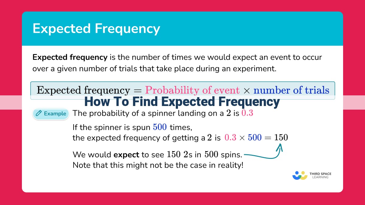
Expected frequency is a value that represents the average number of times an event is expected to occur over a large number of trials in a probability distribution. It is calculated by summing the probability of each possible outcome of an event and multiplying each probability by its corresponding frequency. The sum of the expected frequencies for all possible outcomes should equal the total number of trials. Expected frequency provides information about the likely occurrence of events and helps in understanding the behavior of random variables.
Types of Probability Distributions:
- Define marginal, joint, and conditional probability distributions.
Understanding Probability Distributions: Separating Events and Measuring Outcomes
Probability distributions are the tools we use to understand the likelihood of various events occurring. They allow us to predict outcomes, analyze data, and make informed decisions. Just as a map helps us navigate unfamiliar terrain, probability distributions guide us through the realm of uncertainty.
Types of Probability Distributions: Dissecting the Landscape of Uncertainty
Imagine a glass jar filled with marbles. Each marble has a unique color. The marginal probability distribution tells us the probability of drawing a specific color marble, while the joint probability distribution describes the probability of drawing two or more marbles of specific colors.
Now, let’s add a twist. We’re told that the jar contains only red and blue marbles. The conditional probability distribution comes into play here. It tells us the probability of drawing a red marble given that we know the marble is blue or vice versa.
Marginal Probability Distribution: The Spotlight on Individual Events
The marginal probability distribution shines a light on individual events. It provides a snapshot of the probability of each event occurring independently of any other events. In our marble jar example, the marginal probability of drawing a red marble is simply the number of red marbles divided by the total number of marbles.
Joint Probability Distribution: Capturing the Interplay of Events
The joint probability distribution plays a different role. It considers the probability of multiple events occurring simultaneously. In our marble jar example, the joint probability of drawing a red marble and then a blue marble would be the product of the marginal probabilities of drawing each marble individually.
Conditional Probability Distribution: Unraveling Cause-and-Effect Relationships
The conditional probability distribution paints a more nuanced picture. It helps us understand how the occurrence of one event affects the probability of another. In our marble jar example, the conditional probability of drawing a red marble given that the previous marble drawn was blue would be different from the marginal probability of drawing a red marble.
Understanding these concepts is the key to unlocking the power of probability distributions. They allow us to better understand the world around us, make informed decisions, and navigate the uncertain waters of life. Just as a compass guides a sailor, probability distributions guide us through the sea of uncertainty.
Marginal Probability Distribution:
- Explain how marginal distributions are derived from joint distributions.
- Discuss how they represent the probability of individual events.
Marginal Probability Distributions: Unveiling the Probability of Individual Events
In the realm of probability, events don’t always occur in isolation. Sometimes, we need to consider the interplay between multiple events to make informed decisions. This is where joint probability distributions come into play, capturing the likelihood of two or more events happening simultaneously.
But what if we’re only interested in the probability of a single event, regardless of what other events may be occurring? That’s where marginal probability distributions step in. Derived from joint distributions, marginal distributions reveal the probability of individual events, giving us a clearer picture of the likelihood of their occurrence.
To understand how marginal distributions work, let’s consider a simple example. Imagine a coin toss where the outcome can be either heads or tails. The joint probability distribution of this event would show the probabilities of all possible combinations of outcomes:
| Head | Tails | Probability |
|---|---|---|
| Yes | Yes | 0 |
| Yes | No | 0.5 |
| No | Yes | 0.5 |
| No | No | 0 |
The marginal probability distribution of heads would simply show the probability of getting heads, regardless of the outcome of the tails event:
| Head | Probability |
|---|---|
| Yes | 0.5 |
| No | 0.5 |
Similarly, the marginal probability distribution of tails would show the probability of getting tails, regardless of the outcome of the heads event:
| Tail | Probability |
|---|---|
| Yes | 0.5 |
| No | 0.5 |
By giving us the probability of individual events, marginal probability distributions provide essential insights into the behavior of random variables. They allow us to make informed decisions, predict future outcomes, and gain a deeper understanding of the world around us.
Understanding Probability Distributions: A Guide to Joint Distributions
Imagine you’re planning a romantic getaway with your significant other. You’re torn between a cozy cabin in the mountains or a sandy beach vacation. To make a well-informed decision, you research both options and gather data on weather conditions.
Joint Probability Distribution: Capturing Simultaneous Events
This situation calls for a joint probability distribution, which is a mathematical tool that describes the likelihood of two or more events occurring together. In our example, the joint distribution would show the probability of specific weather conditions for both the mountains and the beach.
A joint distribution is typically represented by a table or a graph. The table assigns a probability to each combination of events, while the graph provides a visual representation of the relationship between the events.
From Joint to Marginal: Uncovering Individual Probabilities
A marginal distribution is a special case of a joint distribution that focuses on the probability of an individual event. In our scenario, the marginal distribution for the mountains would show the probability of each weather condition (e.g., sunny, rain, snow) regardless of the beach conditions.
Obtaining a marginal distribution from a joint distribution is straightforward. Simply sum the joint probabilities for all combinations involving the event of interest. For example, to find the probability of rain in the mountains, we would add up the probabilities of rain in all the combinations where the beach conditions are varied.
Key Takeaways: Unveiling the Power of Joint Distributions
- Joint probability distributions provide a comprehensive view of the likelihood of simultaneous events.
- They are essential for understanding the relationships between multiple variables or events.
- Marginal distributions, derived from joint distributions, reveal the probabilities of individual events.
By mastering the concept of joint probability distributions, you can make informed decisions that account for multiple factors and enhance your understanding of the world around you.
Conditional Probability Distribution: Uncovering Hidden Dependencies
In the realm of probability, the conditional probability distribution holds a special place. It unveils the secrets of events that unfold in the shadow of prior knowledge. Unlike the unconditional world of marginal distributions, the conditional probability distribution captures the intricate dance between one event’s likelihood and the presence of another.
What is Conditional Probability?
Imagine tossing a coin. The marginal probability of getting heads is 0.5, meaning you have a 50% chance of success. But what if we add a twist? Consider a situation where you flip the coin a second time, knowing that the first toss resulted in heads.
The conditional probability of getting heads on the second toss is now different. It’s no longer a simple 0.5. Why? Because the first toss has provided us with a clue that affects the likelihood of the second. The conditional probability distribution captures this dependence, showing us how events shape each other’s probabilities.
Applications of Conditional Probability
The conditional probability distribution is not just a theoretical concept. It has countless practical applications, such as:
- Medical diagnosis: By considering a patient’s symptoms and medical history, doctors can use conditional probability to estimate the likelihood of different diseases.
- Predictive analytics: Companies analyze past data to predict customer behavior. Conditional probabilities allow them to adjust their predictions based on specific customer characteristics or demographics.
- Weather forecasting: Meteorologists use conditional probabilities to refine their predictions, taking into account factors like temperature, humidity, and wind speed.
Example: A Tale of Two Dice
Let’s return to our coin-tossing example. Suppose you flip two coins, one after the other. The conditional probability of getting heads on the second coin is higher if the first coin landed on heads. Similarly, it’s lower if the first coin showed tails.
This is because the first toss provides information about the second. If the first toss was heads, there’s a higher chance of the second coin also being heads. Conversely, if the first toss was tails, the likelihood of the second coin showing heads decreases.
The conditional probability distribution is a powerful tool that unveils the hidden dependencies between events. It’s a bridge between the present and the future, providing us with insights that can inform our decisions and enhance our understanding of the world.
Understanding Probability Distributions and Measures of Central Tendency
Delving into the realm of probability distributions and measures of central tendency is like embarking on an expedition into the intricate workings of probability theory. Let’s navigate through this fascinating landscape, uncovering the secrets of probability distributions and the enigmatic world of expected value, variance, standard deviation, and the enigmatic Z-score.
Probability Distributions: The Essence of Randomness
Just as a myriad of factors influence the outcome of a coin flip, probability distributions model the likelihood of diverse events occurring. They provide a mathematical framework to quantify the chances of various outcomes.
Marginal Probability Distribution: Uncovering Individual Events
Imagine a bag filled with colored marbles. The marginal probability distribution reveals the chances of each color appearing when you draw a marble without peeking. It’s like taking a snapshot of the individual possibilities.
Joint Probability Distribution: Embracing Simultaneity
Now, let’s consider a bag containing marbles of different colors and sizes. The joint probability distribution captures the likelihood of simultaneously drawing specific colors and sizes. It paints a comprehensive picture of multiple events occurring together.
Conditional Probability Distribution: Knowledge as a Guiding Light
Suppose you learn that the first marble drawn was blue. The conditional probability distribution sheds light on the chances of drawing different colors or sizes given this new information. It’s like refining our expectations based on what we already know.
Measures of Central Tendency: Pinpointing the Average
At the heart of understanding data lies the concept of central tendency. These measures help us identify the typical value in a distribution.
Expected Value: The Heart of the Average
The expected value represents the average outcome of an experiment or observation. Think of it as the “fair” value you’d expect to obtain over multiple repetitions. It’s like finding the balance point of a distribution.
Variance and Standard Deviation: Quantifying Spread
The variance measures how scattered data is around the expected value. A higher variance indicates greater dispersion, while a lower variance signifies data clustered close to the average.
The standard deviation is the square root of the variance. It represents the typical distance from the expected value. A smaller standard deviation implies data tightly packed around the average, while a larger standard deviation indicates more spread-out data.
Z-score: Normalizing the Normal
The Z-score transforms data into a standardized form, allowing for easy comparisons. It measures the distance from the expected value in terms of standard deviations. A Z-score of 0 means the data point is exactly the average, while positive and negative Z-scores indicate above or below average values, respectively.
Variance: Measuring the Spread of a Distribution
Variance is a crucial measure that quantifies the dispersion or spread of data points around their central tendency. It measures how scattered a distribution is from its mean, revealing the level of variability within the data.
Variance is calculated by finding the average squared difference between each data point and the mean. This means it accounts for both the magnitude and direction of the deviations from the mean. Higher variance indicates a wider spread of data points, while lower variance suggests data points are clustered more closely around the mean.
The relationship between variance and the mean is vital. Variance is a measure of variability around the mean, capturing how much the data deviates from it. A large mean doesn’t necessarily imply high variance, and vice versa. For example, two distributions with the same mean can have vastly different variances, indicating one group is more spread out than the other.
Standard Deviation: A Measure of Data Dispersion
Standard deviation, rooted in the concept of variance, is a crucial measure of dispersion in statistical analysis. It serves as an indicator of the typical distance of data points from the mean, providing valuable insights into the variability of a dataset.
Visualize a group of students taking a test. The mean score, or average, represents the central point around which the individual scores are distributed. Standard deviation tells us how far, on average, the students’ scores deviate from this central point.
Calculating Standard Deviation
The formula for standard deviation involves calculating the square root of the variance. Variance measures the spread of the data, indicating how far each data point is from the mean. By taking the square root of the variance, we obtain a value that is expressed in the same units as the original data, making it easier to interpret.
Significance of Standard Deviation
Standard deviation is a powerful measure because it enables us to quantify the variability of a dataset. A high standard deviation indicates that the data points are widely spread out from the mean, suggesting a high degree of variability. Conversely, a low standard deviation signifies that the data points are closely clustered around the mean, indicating less variability.
Applications in Real-World Scenarios
Standard deviation finds numerous applications in various fields. In education, it helps teachers assess the performance of students and identify those struggling with the material. In finance, it assists investors in evaluating the risk associated with different investments. In medicine, it provides valuable information about the effectiveness and side effects of treatments.
Standard deviation is an indispensable tool in statistical analysis, providing a quantitative measure of data dispersion. By understanding the concept of standard deviation, we gain a deeper insight into the variability of datasets, enabling us to make informed decisions based on statistical evidence.
Z-score:
- Describe the Z-score as a measure of the distance from the mean in standard deviation units.
- Explain its use in standardizing and comparing data points.
Understanding Z-Scores: A Gateway to Standardizing and Comparing Data
In the realm of statistics, the Z-score emerges as a powerful tool that empowers us to delve into the intricate world of data distributions. This enigmatic measure unravels the mystery of dispersion, providing insights into how data points are dispersed around their central tendency.
Imagine you have a class of students with varying test scores. Some may have excelled, while others may have struggled. The mean, or average score, offers a snapshot of the overall performance. But what if we want to understand how far each student deviates from this average? Enter the Z-score, the unsung hero of data standardization.
The Z-score, denoted as z, measures the distance of a particular data point from the mean in standard deviation units. It essentially translates raw data into a standardized scale, allowing us to compare data points that may have been measured on different scales.
The formula for Z-score is:
z = (x - μ) / σ
where:
- x is the raw data point
- μ is the mean
- σ is the standard deviation
By calculating the Z-score, we transform the data point into a value that indicates how many standard deviations it is away from the mean. A Z-score of 0 represents the mean, while a positive Z-score indicates that the data point is above the mean, and a negative Z-score indicates that it is below the mean.
For instance, a Z-score of 2 means that the data point is two standard deviations above the mean. This suggests that the data point is relatively far from the typical or average value. Conversely, a Z-score of -1 implies that the data point is one standard deviation below the mean, indicating a value that is closer to the lower end of the distribution.
The beauty of Z-scores lies in their ability to facilitate comparisons between data points from different distributions. By standardizing the data, we can make meaningful comparisons even when the original measurements were on different scales. This versatility makes Z-scores indispensable in statistical analysis, hypothesis testing, and data exploration.
Binomial Distribution:
- Define the binomial distribution and its application in modeling success counts.
- Discuss the key parameters involved and provide examples.
Understanding Probability Distributions: The Building Blocks of Statistical Analysis
In the realm of statistics, probability distributions play a pivotal role in modeling the likelihood of events and understanding the underlying patterns in data. They provide a framework for quantifying the uncertainty and variability associated with random phenomena.
Marginal, Joint, and Conditional Distributions
Probability distributions come in three main flavors: marginal, joint, and conditional. A marginal probability distribution represents the likelihood of a single event occurring, while a joint probability distribution describes the probability of multiple events happening simultaneously. A conditional probability distribution, on the other hand, expresses the probability of an event given that another event has already occurred.
Measures of Central Tendency and Dispersion
To summarize and describe probability distributions, statisticians rely on measures of central tendency and dispersion. The expected value, or mean, captures the “average” outcome of the distribution, while the variance measures the spread or variability around the mean. The standard deviation, the square root of the variance, quantifies the typical distance of data points from the mean.
Types of Probability Distributions
The real power of probability distributions lies in their diversity. Different types of distributions model different types of data and phenomena. Some of the most commonly encountered distributions include:
- Binomial Distribution: This distribution is used to model the number of successes in a sequence of independent experiments with a constant probability of success.
- Normal Distribution (Bell Curve): The bell curve is a continuous distribution that describes a wide range of natural and social phenomena. It is characterized by its symmetric, bell-shaped curve.
Binomial Distribution: Modeling Success Counts
The binomial distribution is particularly useful for modeling the number of successes in a sequence of independent experiments. It is characterized by two parameters:
- n: The total number of trials or experiments
- p: The probability of success on each trial
The binomial distribution can be used to answer questions such as “What is the probability of getting exactly 5 heads in 10 coin flips?” or “How many successful experiments do we expect to see in a sample of 20?”
By understanding probability distributions, we gain a deeper insight into the underlying patterns of data. They provide a robust framework for modeling uncertainty, making predictions, and drawing inferences from statistical data.
The Normal Distribution: The Bell Curve of Probability
Imagine a beautiful meadow, where the grass grows in a smooth, bell-shaped curve. This curve mirrors the distribution of data points in the normal distribution, also known as the “bell curve.” It’s a continuous probability distribution that governs a wide range of natural phenomena, from heights of people to IQ scores.
The normal distribution is known for its distinctive bell-shaped curve, which peaks at the mean of the distribution. This mean value represents the average or most typical outcome. The curve gradually tapers off on either side of the mean, indicating that extreme values become increasingly rare.
The normal distribution is characterized by two key parameters: the mean and the standard deviation. The mean, as we’ve established, is the average value. The standard deviation, on the other hand, measures how much the data points spread out around the mean. A smaller standard deviation indicates that the data is more clustered around the mean, while a larger standard deviation suggests a wider spread.
The beauty of the normal distribution lies in its predictable nature. It follows a specific mathematical formula that allows us to calculate the probability of any given outcome. This makes it an invaluable tool in fields such as statistics, quality control, and engineering, where it’s used to make inferences, draw conclusions, and predict future events.
In conclusion, the normal distribution is a powerful tool that helps us understand and interpret data in a meaningful way. Its bell-shaped curve represents the natural tendency of many real-world phenomena to cluster around an average value, with extreme values being less common. By understanding the normal distribution, we can better make sense of the world around us.
Chi-square Distribution: Understanding the “Goodness-of-Fit” Test
Imagine you’re a scientist conducting an experiment. You hypothesize that a new drug will significantly reduce the symptoms of a particular disease. To test this, you administer the drug to a group of patients and track their recovery. However, instead of relying on a simple yes/no answer, you want to assess how closely your observed results fit the expected distribution under the hypothesis. This is where the chi-square distribution comes into play.
The chi-square distribution is a special probability distribution that measures the discrepancies between an observed distribution and an expected distribution. It’s used in statistical tests, such as the goodness-of-fit test, to determine how likely it is that the observed results could have occurred by chance.
The chi-square statistic, denoted by the Greek letter $\chi^2$, is calculated by summing the squared differences between the observed and expected frequencies for each category in the distribution. If the $\chi^2$ value is high, it indicates that the observed distribution is significantly different from the expected distribution, suggesting that the hypothesis may be false or that other factors are at play.
In practice, the chi-square distribution is used in a variety of applications, including:
- Testing whether the proportions of different categories in a sample match the proportions expected under a certain hypothesis.
- Assessing whether a sample comes from a population with a specified distribution (e.g., normal distribution).
- Comparing the variances of two independent samples.
Understanding the chi-square distribution is crucial for researchers and statisticians as it provides a powerful tool for evaluating the fit between observed data and theoretical expectations. By interpreting the chi-square values correctly, we can gain valuable insights into the nature of our data and the validity of our hypotheses.
T-distribution:
- Explain the purpose of the t-distribution when population standard deviation is unknown.
- Discuss its role in hypothesis testing and confidence intervals.
Understanding the T-Distribution: A Lifeline When the Standard Deviation is Unknown
In the realm of statistics, we often encounter situations where we need to draw conclusions or make inferences about a population’s mean value. However, when the population standard deviation is unknown, the regular normal distribution falls short. Enter the T-distribution, a powerful tool that steps in to save the day.
The T-distribution is a bell-shaped distribution similar to the normal distribution, but it has fatter tails, indicating a higher probability of extreme values. These fatter tails arise because the T-distribution is based on a smaller sample size, introducing more uncertainty in the estimation of the population standard deviation.
The T-distribution’s true strength lies in its ability to handle uncertainty. When the sample standard deviation is unknown, the T-distribution provides a more accurate estimate of the population mean than the normal distribution. This makes it the go-to distribution for hypothesis testing and confidence intervals, two essential statistical techniques used to draw inferences about a population.
In hypothesis testing, we use the T-distribution to determine if there is a significant difference between the sample mean and a hypothesized population mean. The T-test statistic measures the distance between the sample mean and the hypothesized mean in terms of standard deviation units. A large T-statistic indicates a greater difference, making it more likely to reject the null hypothesis (the hypothesis that there is no difference).
Confidence intervals are another valuable tool in statistics. They provide a range of plausible values within which the true population mean is likely to lie. The T-distribution allows us to construct confidence intervals even when the population standard deviation is unknown.
In summary, the T-distribution is an indispensable tool for statistical analysis when the population standard deviation is unknown. Its fatter tails and ability to handle uncertainty make it essential for hypothesis testing and confidence intervals. So, the next time you encounter a statistical problem with an unknown standard deviation, remember the trusty T-distribution—it’s your lifeline to reliable inferences.
Diving into the F-Distribution: A Tale of Variance Comparison
In the world of statistics, probability distributions play a crucial role in understanding and interpreting data. Among these distributions, the F-distribution stands out as a powerful tool for comparing the variances of two populations.
What is the F-Distribution?
Imagine you have two groups of data, each representing a different population. The F-distribution helps you determine if these groups exhibit significantly different levels of variation. It quantifies the ratio of the variances of two independent samples and follows a specific probability distribution.
Applications of the F-Distribution
The F-distribution finds wide application in statistical tests, particularly the Analysis of Variance (ANOVA). ANOVA is a technique used to compare the means of multiple groups. By testing whether the variances of these groups are equal, the F-distribution contributes to the overall assessment of whether there are significant differences between the means.
Interpretation of F-Values
When you calculate an F-value, a small value indicates that the variances of the two populations are similar, while a large value suggests they are significantly different. A high F-value implies that one group exhibits much greater variability than the other.
Significance Testing with the F-Distribution
To determine whether the difference in variances is statistically significant, you compare the calculated F-value to a critical value obtained from the F-distribution table. If the F-value exceeds the critical value, it provides evidence that the variances of the two populations are not equal.
The F-distribution is an essential tool in statistical analysis, enabling researchers to compare the variances of two populations. By understanding the concept and applications of the F-distribution, you can effectively interpret data and draw meaningful conclusions about the variability within and between different groups.