Essential Guide: Identifying Conservative Vector Fields
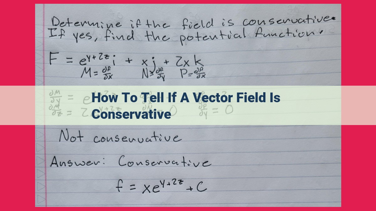
How to Tell If a Vector Field Is Conservative
A conservative vector field can be described as a force field that is path-independent, meaning the work done by the field is independent of the path taken. To determine if a vector field is conservative, examine the following properties:
- Path Independence: The integral of the vector field around any closed curve is zero.
- Closed Curves: The vector field has a potential function, which is a scalar function whose gradient equals the vector field.
- Divergence: The divergence of the vector field is zero, indicating the field has no sources or sinks.
- Exact Differentials: The vector field can be expressed as the gradient of some scalar potential function, known as an exact differential.
- Irrotational: The curl of the vector field is zero, implying the field is free of rotational motion.
Unveiling the Essence of Conservative Vector Fields
In the realm of vector calculus, conservative vector fields hold a captivating allure. These special vector fields possess an intriguing property that sets them apart from their ordinary counterparts. In this blog post, we embark on a journey to unravel the secrets of conservative vector fields, guiding you through the fundamental concepts that define their unique behavior.
Unveiling the Concept of Conservative Vector Fields
At its core, a conservative vector field is a vector field that can be expressed as the gradient of a scalar function. Imagine a scalar function as a landscape, with its values representing the height at each point. The gradient of this function, which is a vector field, points in the direction of the steepest ascent.
Consider a hiker traversing this landscape, represented by a conservative vector field. The hiker’s path follows the gradient lines of the function, always ascending towards higher values. Crucially, the hiker’s path is path independent. Regardless of the meandering route they choose, the total change in elevation, or the line integral of the vector field around a closed curve, is always zero. This property, known as the Gradient Theorem, is a defining characteristic of conservative vector fields.
Potential Functions and Closed Curves
The scalar function associated with a conservative vector field is known as a potential function. It represents the gravitational potential energy or electrical potential, depending on the context. The Gradient Theorem implies that the line integral of a conservative vector field around any closed curve is zero because the potential function’s value at the starting and ending points is the same. Hence, the work done by the vector field over a closed loop is zero.
Unveiling Divergence and Irrotationality
Conservative vector fields also possess two other remarkable properties. First, they are always divergence-free. Divergence measures the outward flux of a vector field from a point, and for conservative vector fields, this flux is always zero. This means that the vector field neither creates nor destroys sources or sinks of the field.
Second, conservative vector fields are irrotational. The curl of a vector field measures its circulation around a point. For conservative vector fields, the curl is always zero, indicating that the vector field has no rotational component. In other words, the vector field is in a state of pure “curliness” or circulation.
Conservative vector fields, with their remarkable properties, play a significant role in various scientific and engineering disciplines. They offer insights into the behavior of electric and gravitational fields, fluid dynamics, and heat transfer. By understanding the intricate nature of conservative vector fields, researchers and practitioners gain a deeper grasp of the physical phenomena that shape our world.
The Gradient Theorem: Unlocking the Secrets of Conservative Vector Fields
In the fascinating world of vector calculus, conservative vector fields reign supreme, possessing a unique and remarkable property. The Gradient Theorem reveals this hidden truth: when you embark on a journey around a closed curve in the presence of a conservative vector field, the integral of that field along your path will always vanish to zero.
This astonishing result holds immense significance. It implies that the work done by a conservative vector field is independent of the path taken. In other words, no matter how you maneuver around a closed loop, the total amount of work done remains the same.
The Gradient Theorem is not merely an abstract mathematical concept; it has profound implications for the practical world. Imagine a hiker traversing a treacherous mountain trail in search of a hidden summit. The hiker’s elevation gain, represented by a conservative vector field, is independent of the specific route taken. Whether they ascend via a winding path or a treacherous scramble, the effort expended remains unchanged.
This path independence has far-reaching applications in fields such as electromagnetism and fluid dynamics. In electromagnetism, conservative vector fields represent the force fields surrounding electric charges. The Gradient Theorem ensures that the work done by these forces is independent of the path taken by an electron or any charged particle.
In fluid dynamics, conservative vector fields describe the velocity fields of fluids. The Gradient Theorem implies that the circulation of a fluid around a closed loop is zero. This concept is crucial for understanding the flow patterns and energy conservation in fluid systems.
The Gradient Theorem is a powerful tool that unlocks the secrets of conservative vector fields. Its implications extend far beyond the realm of mathematics, providing insights into the workings of our physical world.
Path Independence: A Unique Property of Conservative Vector Fields
In the realm of vector calculus, conservative vector fields stand out with a remarkable characteristic known as path independence. This property sets them apart from other vector fields and has profound implications for solving problems involving these special fields.
Defining Path Independence
Path independence refers to the fact that for a conservative vector field, the line integral along any path connecting two points is the same, regardless of the actual path taken. In other words, the work done by the field along different paths is identical.
Significance of Path Independence
This property has tremendous implications for solving problems involving conservative vector fields. For instance, when calculating the work done by a conservative field in moving a particle between two points, we can choose any convenient path and be assured of obtaining the same result.
Additionally, path independence allows us to define a scalar function called a potential function, whose gradient is equal to the conservative vector field. This potential function provides a powerful tool for solving problems, as it allows us to calculate the work done by the field by simply evaluating the difference in the potential function between the starting and ending points.
Practical Applications
Path independence finds applications in various fields of physics and engineering. For example, in electromagnetism, it enables us to calculate the work done by an electric field in moving a charge between two points without regard to the specific path taken. Similarly, in fluid mechanics, path independence allows us to determine the work done by a pressure gradient in moving a fluid parcel.
The path independence of conservative vector fields is a fundamental property that simplifies the analysis and solution of problems involving these fields. It empowers us with the ability to calculate the work done and identify potential functions, making conservative vector fields invaluable tools in a wide range of scientific and engineering applications.
Closed Curves and Conservative Vector Fields
In the realm of vector calculus, conservative vector fields play a pivotal role. They possess a remarkable property that sets them apart from other vector fields: they can be expressed as the gradient of a scalar function, also known as a potential function. This connection between vector fields and scalar functions unlocks a powerful theorem known as the Gradient Theorem.
The Gradient Theorem, a cornerstone of vector calculus, asserts that the integral of a conservative vector field around a closed curve is zero. A closed curve is essentially a loop that begins and ends at the same point. The significance of this theorem lies in its ability to determine whether a vector field is conservative.
Let’s imagine ourselves walking along a closed curve, like a circular path around a park. If the vector field we encounter is conservative, the integral of the vector field around this closed curve will vanish. This result holds true because the potential function associated with the vector field increases as we walk along the path, and then decreases as we return to the starting point. The net change in the potential function over the closed loop is zero, which translates to a zero integral.
Conversely, if the integral of the vector field around a closed curve is not zero, then the vector field cannot be conservative. This is because a non-zero integral would indicate that the potential function is changing as we traverse the closed curve, implying that the vector field cannot be derived from a potential function.
The Gradient Theorem and the concept of closed curves provide a crucial tool for understanding and identifying conservative vector fields. They pave the way for further exploration of the interplay between vector fields and scalar functions, unlocking insights into the behavior of forces, fields, and flows in the physical world.
Divergence and Conservative Vector Fields
Imagine you’re strolling through a bustling city, navigating the myriad streets and avenues. Suddenly, you notice a peculiar pattern: the density of pedestrians seems to vary from block to block. In crowded areas, the flow of people is like a rushing river, while in quieter streets, it’s a mere trickle. This variation in “density” is an example of a fundamental concept in vector calculus: divergence.
Divergence Defined:
Divergence is a mathematical operator that measures the “spreadiness” of a vector field at a particular point. It quantifies how much the vector field is “diverging” or “converging” as you move around the point.
Relationship to Conservative Vector Fields:
Conservative vector fields are special types of vector fields that can be represented as the gradient of a scalar function. This scalar function, often called a potential function, is like a “height” field: it assigns a value to each point in space, indicating how “elevated” that point is.
The divergence of a conservative vector field is always zero. This means that conservative vector fields are always divergence-free.
Proof:
To prove this, we use the product rule for the gradient of a scalar function f:
∇ · (∇f) = ∂²f/∂x² + ∂²f/∂y² + ∂²f/∂z²
Since f is a scalar function, all its second partial derivatives are equal. Therefore, the divergence of ∇f is always zero:
∇ · (∇f) = 0
Implications:
The divergence-free nature of conservative vector fields has important implications. It means that there are no sources or sinks within the vector field. In other words, the vector field cannot create or destroy anything as you move along it. This property is essential for applications in electromagnetism and fluid dynamics.
Exact Differentials
- Define an exact differential and explain how it is related to conservative vector fields.
- Show that conservative vector fields are always given by exact differentials.
Exact Differentials: The Key to Conservative Vector Fields
In the realm of vector calculus, a conservative vector field is like a well-behaved force field where the work done in moving along a path is independent of the path taken. This remarkable property arises from a fundamental relationship between conservative vector fields and a mathematical concept known as exact differentials.
Defining Exact Differentials
An exact differential is a special type of function whose differential (the derivative of the function with respect to each variable) forms a conservative vector field. In other words, if we have a function f(x, y, z), its exact differential is given by:
df = ∂f/∂x dx + ∂f/∂y dy + ∂f/∂z dz
where ∂f/∂x, ∂f/∂y, and ∂f/∂z are the partial derivatives of f.
Conservative Vector Fields as Exact Differentials
The essence of this relationship is that every conservative vector field can be expressed as the gradient of an exact differential. In mathematical terms:
F = ∇f
where F is the conservative vector field and f is its scalar potential (the exact differential).
Significance of Exact Differentials
This connection between conservative vector fields and exact differentials has profound implications:
- Path Independence: The work done by a conservative vector field around a closed path is zero, regardless of the path taken. This is a direct consequence of the fact that the integral of an exact differential around a closed curve is zero.
- Closed Curves: A vector field is conservative if and only if its line integral around every closed curve is zero. This provides a powerful test for determining if a vector field is conservative.
Exact differentials serve as a crucial bridge between conservative vector fields and the powerful tools of calculus. By understanding their relationship, we gain insights into the nature of force fields, potential energy, and the elegant properties of conservative systems.
Conservative Vector Fields: A Journey into Rotational Harmony
As we explore the fascinating realm of vector fields, we encounter a special class known as conservative vector fields. These fields possess a remarkable property that sets them apart from their rotational counterparts: they are irrotational.
What is the Curl of a Vector Field?
The curl of a vector field F is a vector that describes the field’s rotation at a given point. It measures the tendency of the field to “twist” around that point.
Conservative Vector Fields and Irrotationality
Intriguingly, conservative vector fields are always irrotational. This means that the curl of a conservative vector field is always zero. In other words, conservative vector fields do not rotate.
Why Are Conservative Vector Fields Irrotational?
The irrotationality of conservative vector fields can be proven mathematically. Consider a closed curve C in a conservative vector field F. The Gradient Theorem states that the integral of F around C is zero.
If F were rotational, meaning it had a nonzero curl, then the integral around C would not be zero. This is because the curl measures the rotation of F along the curve, and a positive curl would indicate a nonzero net rotation, resulting in a nonzero integral.
Implications of Irrotationality
The irrotational nature of conservative vector fields has important implications. Firstly, it simplifies the analysis of these fields. Since they do not rotate, their behavior is more predictable and easier to understand.
Secondly, irrotationality is closely related to the concept of potential functions. A conservative vector field can be expressed as the gradient of a scalar function known as its potential function. The potential function provides an alternative way to represent the vector field, often making it easier to solve problems involving it.
In summary, conservative vector fields are a special type of vector field that exhibit a remarkable property: they are always irrotational. This means that they do not rotate and can be described by a potential function. The irrotationality of conservative vector fields simplifies their analysis and underscores their fundamental role in the study of vector fields.