Direction Fields For Differential Equations: Visualizing Solutions

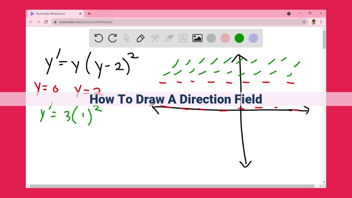
To draw a direction field, first choose a set of points in the plane. At each point, draw a short line segment with slope equal to the value of the differential equation at that point. Connect nearby line segments to form a continuous field of lines. This field represents the direction of the solution to the differential equation at each point in the plane.

Understanding Direction Fields: A Sneak Peek into the Heart of Differential Equations

Unveiling the Plot: What are Direction Fields?

Imagine you’re a hiker navigating a treacherous landscape. Direction fields are like maps that guide you through the terrain of differential equations. They’re a graphical representation of the equation’s solutions, revealing how the slope of the solution changes as you move along the path.

Unraveling the Clues: Slope Fields, Isoclines, and Singular Points

Direction fields are made up of three key elements:

• Slope fields: These are collections of short lines that indicate the slope of the solution at each point, creating a visual tapestry of the equation’s behavior.
• Isoclines: Lines that connect points where the slope is the same, guiding you along paths of consistent gradient.
• Singular points: Special points where the slope is undefined, giving you clues about intriguing dynamics in the solution.

Significance Unveiled: The Power of Direction Fields

These elements work together to paint a vivid picture of the differential equation, allowing you to:

• Identify areas where the solution is increasing or decreasing rapidly.
• Spot potential points of instability or equilibrium.
• Gain insights into the overall behavior of the solution, even without solving the equation explicitly.

Techniques for Drawing Direction Fields: A Detailed Exploration

Drawing direction fields is a powerful tool for visualizing and understanding differential equations. Two primary techniques are commonly employed: Euler’s method and the analytical method.

Euler’s Method

Euler’s method is a numerical approach that approximates the solution of a differential equation over a sequence of steps. It involves using the equation’s slope to estimate where the solution goes next. Starting with an initial point, we calculate the slope using the differential equation at that point. This slope gives us the direction of the tangent line, which leads us to the next point on the solution curve. This process is repeated, generating a series of points that approximate the actual solution.

Analytical Method

The analytical method is more direct and involves solving the differential equation for the slope at each point. By substituting a given value of the independent variable into the equation, we can calculate the corresponding slope. This allows us to construct the direction field without the need for iterative approximations like Euler’s method.

Understanding the Slope Field

Both techniques help us create a slope field. The slope field is a visual representation of the direction of the solution at every point in a given region. At each point, the slope or direction is indicated by a short line segment. By studying the slope field, we can gain insights into the behavior of the differential equation. For instance, areas with consistent slopes suggest regions where the solution is changing gradually. Abrupt changes in slope indicate points of rapid transition or singularities.

Combining Euler’s Method and Analytical Approach

Euler’s method is particularly useful for understanding the direction field qualitatively, while the analytical method provides more accurate information about the slopes. By combining these methods, we can gain a deeper understanding of the differential equation and its behavior.

Drawing direction fields is a crucial skill for visualizing and analyzing differential equations. By mastering Euler’s method and the analytical method, you can effectively construct slope fields, providing valuable insights into the behavior of solutions and their characteristics.

Interconnected Concepts: Unveiling the Relationships in Direction Fields

In the realm of direction fields, a profound interplay exists between slope fields, isoclines, singular points, and Euler’s method. These concepts intertwine to provide a comprehensive understanding of the behavior of differential equations.

Slope fields represent the direction of the solution curves, while isoclines show lines of constant slope. By analyzing these slope fields, we can identify areas where the slope is consistent, indicating stable solutions. Conversely, abrupt changes in the slope indicate potential solutions with rapid changes.

Singular points are special points where the slope is undefined or zero. These points can signify equilibria, where the solution remains constant, or bifurcations, where the solution exhibits different behaviors depending on the initial conditions.

Euler’s method is a numerical technique for approximating the solutions of differential equations. By applying Euler’s method, we can generate approximate slope fields and identify regions of consistency and abrupt changes, helping us to unravel the hidden dynamics of the system.

By comprehending these interconnected concepts, we gain a deeper appreciation for the behavior and characteristics of differential equations. Understanding the interplay between slope fields, isoclines, singular points, and Euler’s method empowers us to visualize and analyze the solutions, gaining valuable insights into the underlying dynamics of complex systems.

Contextualizing with Differential Equations

Understanding direction fields is crucial for visualizing the behavior of differential equations. These graphical representations provide invaluable insights into the solutions of these equations and their characteristics. By mapping out the slopes of solutions at every point in the plane, direction fields allow us to intuitively grasp the flow of solutions and identify areas of interest.

Slope fields, the most common type of direction field, depict the tangent lines to the solution curves of differential equations. By examining the direction of these slopes, we can determine the increasing and decreasing behavior of solutions. For example, if the slopes are generally upward, the solutions are increasing, while downward slopes indicate a decrease.

Additionally, direction fields reveal the presence of isoclines, curves along which the slopes are constant. Isoclines can help us locate equilibrium points, where the solution remains constant, and identify regions where solutions exhibit similar behavior. Understanding the relationship between slope fields, isoclines, and solutions is essential for interpreting the behavior of differential equations.

By drawing direction fields, we can visualize the qualitative behavior of solutions without explicitly solving the equation. This can be particularly useful for complex differential equations where analytical solutions may be difficult or impossible to obtain. Direction fields provide a graphical representation that allows us to make informed predictions about the solutions and their properties, guiding our understanding and future investigations.

Applications and Examples

• Provide real-world examples of where direction fields are used, such as population growth models.
• Guide readers through the process of drawing and interpreting direction fields for specific equations.

Applications and Examples of Direction Fields

In the realm of mathematics, direction fields play a crucial role in visualizing the behavior of differential equations. These graphical representations provide valuable insights into the solutions of differential equations, offering a deeper understanding of their characteristics and applications.

One prominent application of direction fields lies in the modeling of population growth. Imagine a population of organisms growing at a rate proportional to its size. We can represent this scenario using a differential equation of the form:

$\frac{dN}{dt} = kN$

where (N) represents the population size, (t) denotes time, and (k) is the growth rate.

By constructing a direction field for this equation, we can visualize the slope of the solution curves at each point in the phase plane. Each point on the field corresponds to a particular population size and growth rate. The direction of the slope at that point indicates the rate of change of the population over time.

Another example where direction fields prove useful is in understanding the behavior of chemical reactions. Consider a reaction between two chemicals, (A) and (B), where the concentration of (A) changes over time according to the following differential equation:

$\frac{dA}{dt} = -kA^2B$

where (k) is the reaction rate constant.

The direction field for this equation depicts the slope of the solution curves at various concentrations of (A) and (B). The slopes indicate the rate at which (A) is consumed or produced in the reaction, providing insights into the kinetics of the chemical process.

In practice, drawing direction fields can be a valuable tool for scientists, engineers, and researchers across various disciplines. They aid in the qualitative analysis of differential equations, helping experts make informed predictions about system behavior and identify potential areas of interest for further investigation.

Advanced Techniques and Further Exploration

Embarking on the journey of differential equations and direction fields, you’re armed with a solid foundation. Now, let’s venture into advanced techniques to expand your understanding.

Numerical Integration for Enhanced Accuracy:

Numerical integration methods, such as the Runge-Kutta method, provide a more precise approach to approximating solutions to differential equations. By breaking down the equation into smaller increments, numerical integration offers greater accuracy in capturing intricate details of the solution.

Graphing Software: A Visual Aid to Complexity:

Harness the power of graphing software to visualize direction fields and explore complex equations in an interactive environment. Software like MATLAB, Python’s SciPy library, and GeoGebra facilitate the creation of dynamic direction fields, allowing you to observe the behavior of differential equations in real time.

Interactive Simulations: Experiential Learning:

Immerse yourself in the world of differential equations through engaging online simulations. Interactive simulations provide a hands-on experience, enabling you to adjust parameters and observe the corresponding changes in direction fields and solutions. This experiential learning enhances your comprehension and deepens your understanding.

Further Exploration: Uncharted Territories:

Expand your knowledge by exploring additional resources that delve deeper into differential equations and direction fields. Online repositories offer a wealth of interactive simulations, tutorials, and research papers. Engage in discussions on forums and connect with fellow enthusiasts to broaden your perspectives and foster your curiosity.