Determining Upper And Lower Limits: A Statistical Guide To Accuracy And Confidence

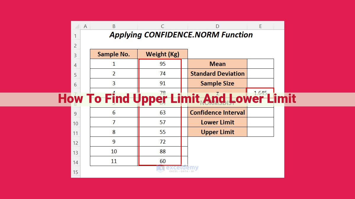
To find upper and lower limits, understand absolute error and its role in measuring accuracy. Use bounding intervals to establish a range of values within which the true value is likely to lie. Consider the maximum and minimum values to determine the extent of the data set. Employ statistical concepts like standard deviation and T-distribution to calculate confidence intervals and assess statistical significance. This process allows for the determination of the upper and lower bounds with a specified level of certainty.

Understanding Absolute Value:

• Definition and purpose of absolute value
• Its use in determining distance between numbers on a number line
• Related concepts: sign, magnitude, and negative value

Understanding the Essence of Absolute Value

In the realm of mathematics, we often encounter numbers that reside far from the tranquil shores of zero. These numbers, both positive and negative, carry a magnitude that reflects their distance from the numerical equator. Enter absolute value, a concept that sheds light on this numerical distance, transforming the vast expanse of numbers into a navigable landscape.

Absolute value, symbolized by vertical bars (| |), captures the magnitude of a number without regard to its sign. It transforms negative numbers into their positive counterparts, revealing their true size. For instance, the absolute value of -5 is 5, while the absolute value of 7 remains 7. This powerful operator allows us to focus on the distance from zero, disregarding the direction (positive or negative) along the number line.

In this mathematical adventure, we explore the fascinating world of absolute value. We unravel its role in measuring the distance between numbers, revealing its connection to sign, magnitude, and negative values. Join us as we delve into the enchanting realm of absolute value, a concept that empowers us to navigate the enigmatic world of numbers.

Absolute Error: Measuring the Accuracy of Measurements

Imagine you’re measuring the height of a skyscraper using a measuring tape. Even with the most careful measurements, there is a chance that you might not get it exactly right. This slight deviation from the true height is known as measurement error.

To quantify this error, we use absolute error. Absolute error is simply the distance between the measured value and the true value. The smaller the absolute error, the more accurate the measurement.

Absolute error is particularly important in situations where accuracy is crucial. In engineering, construction, and scientific research, even small errors can have significant consequences. Understanding absolute error can help us make more informed decisions about the reliability of our measurements.

For example, if a medical diagnosis is based on a measurement with a large absolute error, it could lead to incorrect treatment or missed diagnoses. In finance, inaccurate measurements of financial data can result in poor investment decisions. Therefore, it is essential to be aware of the potential for measurement error and to take steps to minimize its impact.

Absolute Error vs. Precision

Precision measures how consistent a set of measurements is, while accuracy measures how close the measurements are to the true value. A measurement can be precise without being accurate, and vice versa.

For example, if you measure the height of a skyscraper multiple times and get the same result each time, your measurements are precise. However, if the result is consistently 10 meters off from the true height, your measurements are not accurate.

Understanding both precision and accuracy is important for interpreting measurement results. A high degree of precision does not necessarily imply a high degree of accuracy, and a low degree of precision does not necessarily imply a low degree of accuracy.

Bounding Intervals and Confidence Intervals: Navigating Uncertainty in Statistics

In the realm of statistics, uncertainty often accompanies our data. We strive to make inferences about the underlying population based on limited samples, but how can we quantify and present this uncertainty effectively? Enter the concepts of bounding intervals and confidence intervals.

Defining Bounding Intervals:

A bounding interval provides an upper and lower bound within which we can expect or are confident that a given parameter or value falls, based on the available data. It is like constructing a “box” around an uncertain number or value.

Utilizing Confidence Intervals and Bounding Intervals:

Confidence intervals are a specific type of bounding interval that indicate the range of possible values for a population parameter, such as a mean or proportion, with a specified level of confidence. For instance, a 95% confidence interval means that we are 95% confident that the true parameter lies within that range.

Complementing Each Other:

Bounding intervals and confidence intervals play complementary roles in statistical analysis. Bounding intervals offer a broader range within which the parameter may exist, while confidence intervals provide a more specific estimate with a quantifiable level of certainty.

Connecting Concepts:

• Confidence level: The specified probability that the true parameter lies within the confidence interval.
• Error bars: Visual representations of bounding intervals or confidence intervals.
• Statistical analysis: The process of using data and statistical techniques to make inferences or draw conclusions about a population.

By understanding bounding intervals and confidence intervals, we gain valuable insights into the uncertainty associated with statistical inferences. These concepts empower us to make informed decisions, communicate results effectively, and navigate the uncertainties that are inherent in statistical investigations.

Precision, Accuracy, and Maximum and Minimum Values: The Cornerstones of Data Analysis

In the realm of data analysis, precision and accuracy are often conflated. However, understanding the distinction between these two concepts is crucial for interpreting and communicating data effectively.

Precision refers to the closeness of measurements to each other. It indicates how consistently a measuring instrument or method reproduces the same result. High precision implies that repeated measurements tend to be very similar.

Accuracy, on the other hand, measures how close a measurement is to the true value. It reflects the closeness of the data to the actual reality it represents. High accuracy means that the measurements are generally very close to the true values.

To illustrate the difference, consider a dartboard. Throwing darts repeatedly at the same spot demonstrates high precision, as the darts are consistently clustered close together. However, if the spot you’re aiming at is not the bullseye, your darts may be precise but not accurate.

Maximum and minimum values are also vital in characterizing a data set. The maximum value represents the largest observed value, while the minimum value is the smallest. These values define the range of the data, indicating the extent of its spread.

Outliers, extreme values that lie far from the rest of the data, can significantly influence the maximum and minimum values. They can also distort the overall impression of the data. Therefore, it’s important to identify and handle outliers appropriately in your data analysis.

Understanding precision, accuracy, and maximum and minimum values is fundamental for interpreting data correctly. By considering these factors, you can gain valuable insights into the consistency and reliability of your data and draw more informed conclusions.

Hypothesis Testing: Unveiling the Significance in Statistics

In the realm of data analysis, hypothesis testing stands as a cornerstone, empowering us to evaluate claims and make informed decisions. It’s a statistical technique that transforms mere data into meaningful insights, allowing us to unravel hidden truths and draw confident conclusions.

At the heart of hypothesis testing lies the null hypothesis. This is a statement that assumes there is no significant difference or effect. On the other hand, the alternative hypothesis proposes that a meaningful difference or effect exists. Our goal is to determine whether the data supports the null hypothesis or suggests an alternative reality.

To guide our decision, we employ the concept of significance level, denoted by the Greek letter alpha (α). This value represents the probability of rejecting the null hypothesis when it is actually true. Typically, we set alpha at a conventional value like 0.05, meaning we are willing to accept a 5% chance of making a false positive error (rejecting the null hypothesis when it is true).

The p-value is another crucial element in hypothesis testing. It measures the probability of obtaining a result at least as extreme as the one observed, assuming the null hypothesis is true. A low p-value (less than alpha) indicates that the observed result is unlikely under the null hypothesis, leading us to reject it in favor of the alternative hypothesis.

Hypothesis testing is a powerful tool that allows us to make informed decisions based on data. It helps us distinguish between random fluctuations and meaningful patterns, unlocking the insights hidden within our data and illuminating the path towards evidence-based conclusions.

Standard Error, Standard Deviation, and T-Distribution: Unlocking Statistical Insights

In the realm of statistics, three key concepts – standard error, standard deviation, and the T-distribution – play a crucial role in helping us understand and analyze data. Let’s delve into each of these concepts, unraveling their significance and interdependence.

Standard Error: The Estimated Standard Deviation

Imagine you have a population of data, but it’s impractical to measure every single value. Enter standard error, a valuable tool that allows us to estimate the true population standard deviation based on a sample of the data. Standard error is the standard deviation of the sampling distribution, which is the distribution of all possible sample means that could be drawn from the population.

Standard Deviation: Measuring Data Spread

Standard deviation is a measure of how much data is spread out around the mean. A smaller standard deviation indicates that the data is clustered closer to the mean, while a larger standard deviation suggests a wider spread. Understanding the standard deviation helps us gauge the variability within a data set and make informed inferences.

T-Distribution: Stepping Up for Small Sample Sizes

In hypothesis testing, when we have a small sample size (n < 30), the T-distribution comes into play. The T-distribution resembles the normal distribution but is slightly more spread out. It allows us to make inferences about the population mean when our sample size is too small to assume a normal distribution. By using the T-distribution, we can calculate the critical value to determine whether our sample mean is significantly different from the hypothesized mean.

Interplay of the Trio

These three concepts are intricately intertwined. Standard error provides an estimate of the standard deviation for a sample, which in turn helps us determine the spread of the data. The T-distribution allows us to make inferences about the population mean even with small sample sizes. By understanding their interdependence, we gain a deeper comprehension of statistical analysis and can make more informed decisions based on data.

Type I and Type II Errors: The Pitfalls of Hypothesis Testing

When conducting hypothesis testing, researchers aim to draw conclusions about a larger population based on a sample. While hypothesis testing provides valuable insights, it’s essential to acknowledge the potential for errors. Type I and Type II errors are two such errors that can arise in the process.

Consequences of Type I and Type II Errors

Type I error (false positive) occurs when you reject the null hypothesis even though it’s true. This mistake leads to incorrectly concluding that a significant difference exists when, in reality, there is none. The consequences can be severe, such as implementing ineffective treatments or policies based on erroneous findings.

Type II error (false negative), on the other hand, occurs when you fail to reject the null hypothesis when it’s false. This mistake leads to missing a real difference and failing to take appropriate action. Type II errors are often more costly, as they can lead to missed opportunities or ineffective interventions.

Controlling the Risk of Errors

To mitigate the risk of Type I and Type II errors, researchers use significance level (alpha level) and power analysis.

Significance level is the probability of rejecting the null hypothesis when it’s true. By setting a low alpha level (e.g., 0.05), researchers reduce the chance of committing a Type I error. However, this also increases the chance of committing a Type II error.

Power analysis estimates the probability of detecting a real difference, given the sample size and effect size. By increasing power, researchers can reduce the risk of Type II errors. A higher power indicates a greater ability to detect a difference if it exists.

Related Concepts

• False positive: An incorrect conclusion that a significant difference exists.
• False negative: An incorrect conclusion that no significant difference exists.
• Alpha level: The probability of committing a Type I error.
• Power: The probability of detecting a real difference, given the sample size and effect size.